 DanFin
Predicting Volatility, Not Direction
In short
- Yesterday's return tells you very little about tomorrow's direction, but a lot about how big tomorrow's move might be. The size of moves persists; the direction mostly does not.
- That persistence, called volatility clustering, is what makes volatility useful for one job: deciding how much risk to take, not which way to bet.
- Inverse-volatility sizing shrinks a position when estimated volatility rises and allows a larger one when it falls, subject to a cap.
- In a five-asset trend example, the volatility-sized portfolio earned more, but mostly because it used more exposure. Matched to the same realized risk, it still had a better return-to-risk profile and a shallower drawdown.
- This is one historical sample with costs excluded, and the wider research is mixed. It shows volatility sizing can help; it does not prove it always does.
Most traders want to predict whether the next move will be up or down. Financial data are often more helpful for a different question: how large might the next move be? Daily direction has little reliable short-term memory, but the magnitude of returns often does. Large moves tend to cluster near other large moves, and calm periods tend to be followed by calmer ones. That effect, volatility clustering, is one of the best-established features of financial markets, and it changes what you can realistically do with a forecast.
Direction asks: should the position be long or short?
Volatility asks: how much risk should the position take?
Claim your spot on the waitlist
I am releasing one of my trading strategies shortly. Join the waitlist and receive a discount at launch.
Claim your spot →Direction and volatility are different forecasting problems
In the S&P 500 check behind this research, the lag-one daily return autocorrelation (how much one day's return relates to the next) was about −0.10. That points to only a small tendency toward a next-day reversal, and its practical explanatory power is tiny: squaring the correlation leaves roughly 1% of return variation explained.
So it is too strong to say yesterday tells you nothing, but accurate to say yesterday's return by itself contains little reliable information about tomorrow's direction. The magnitude of returns behaves completely differently. In the same check, the autocorrelation of absolute daily returns (a proxy for the size of the move, ignoring its sign) was about +0.66. That is a strong, persistent signal: a volatile day is very likely to be followed by another volatile day, and a calm day by another calm one. Direction is close to a coin flip; the size of the move clearly is not. That gap is the whole point, and it is why volatility, rather than direction, is what you can lean on for risk models, position sizing and portfolio overlays.
Why this matters for trading
Volatility does not tell you which direction to take. It helps estimate the risk of being wrong, which matters in swing trading, systematic strategies and intraday prop-firm trading alike. A fixed number of contracts does not create fixed risk: one NQ contract in a calm session has a very different return distribution from one NQ contract in a wild one, and the same is true for daily swing positions across asset classes. Volatility-based sizing is therefore best understood as a risk-allocation tool, not a directional signal.
What volatility-based position sizing does
A directional strategy decides whether to be long, short or flat. A sizing rule decides how large that position should be. A basic inverse-volatility rule is:
If estimated volatility rises, the position is cut; if it falls, the strategy can take a larger position, usually up to a leverage cap. In practice you still have to turn that multiplier into an actual quantity for your instrument and stop, which is what a position size calculator does.
| Estimated annualized volatility | Position multiplier |
|---|---|
| 10% | 1.00× |
| 20% | 0.50× |
| 40% | 0.25× |
| 5% | 2.00× before any cap |
Why a multi-asset portfolio is a better demonstration
A single-asset backtest can mislead. If the volatility-sized version has a smaller drawdown, that may simply be because it held less average exposure. A diversified portfolio is a stronger test because volatility sizing does two jobs at once: it changes total exposure through time, and it redistributes risk across assets with different volatility levels. Equal capital does not create equal risk. A 20% allocation to oil can contribute far more portfolio volatility than a 20% allocation to Treasury bonds, and inverse-volatility scaling stops the most volatile sleeve from dominating the whole book.
The strategy test used as the example
To show the idea clearly, the example uses a research-inspired time-series momentum framework based on Moskowitz, Ooi and Pedersen (2012): look at an instrument's own trailing 12-month return, go long next month if it was positive, short if it was negative, and scale position size inversely to estimated volatility. The original paper spans many futures contracts; this is a smaller, more transparent adaptation with five ETF proxies across asset classes.
| Symbol | Exposure |
|---|---|
| IVV | US equities / S&P 500 sleeve |
| TLT | Long-duration US Treasury bonds |
| GLD | Gold |
| USO | Oil |
| DBA | Agricultural commodities |
The data came from the PortBench Market Base Dataset, and the active strategy sample ran from 1 February 2016 through 31 December 2025.
Portfolio rules
The fixed equal-capital version simply weights each asset by its momentum direction:
The volatility-sized version scales each asset by an inverse-volatility multiplier:
Volatility was estimated from exponentially weighted daily returns (a moving average that leans on recent data) using a 60-day centre of mass, and the per-asset multiplier was capped at 2×.
Were the assets actually unrelated?
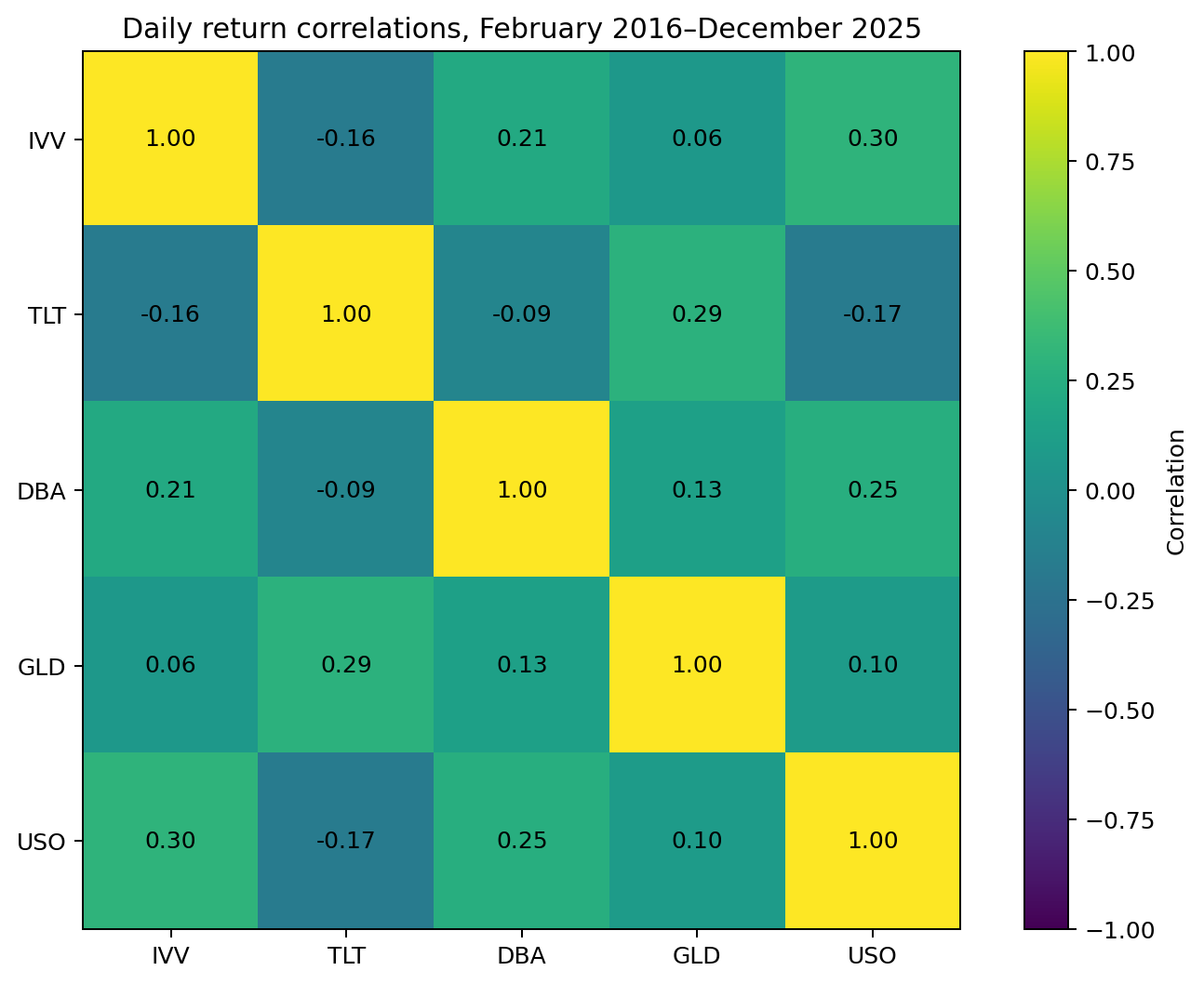
Not completely. "Low-correlated" is more accurate than "uncorrelated." During the active sample, observed daily correlations ranged from about −0.17 to +0.30, still far more diversified than holding several equity indices.
| Pair | Daily return correlation |
|---|---|
| IVV–TLT | −0.16 |
| TLT–USO | −0.17 |
| IVV–GLD | +0.06 |
| GLD–USO | +0.10 |
| IVV–USO | +0.30 |
| TLT–GLD | +0.29 |
Raw portfolio results
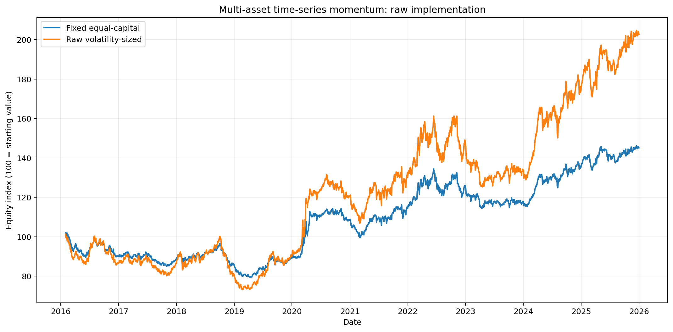
The first comparison uses the two strategies exactly as constructed: the fixed equal-capital portfolio and the raw volatility-sized portfolio.
| Metric | Fixed equal-capital | Raw volatility-sized |
|---|---|---|
| CAGR | 3.71% | 7.31% |
| Annualized volatility | 9.72% | 15.02% |
| Sharpe ratio (0% cash) | 0.44 | 0.55 |
| Maximum drawdown | −22.31% | −27.85% |
| Ending equity index | 145.1 | 202.7 |
| Average gross exposure | 1.00× | 1.82× |
| Maximum gross exposure | 1.00× | 1.98× |
The raw volatility-sized strategy earned more, but it also used significantly more gross exposure (total position size relative to the account). A higher return is not by itself evidence of a better risk process: a strategy that takes more total risk can easily produce a higher return.
Equal-risk comparison
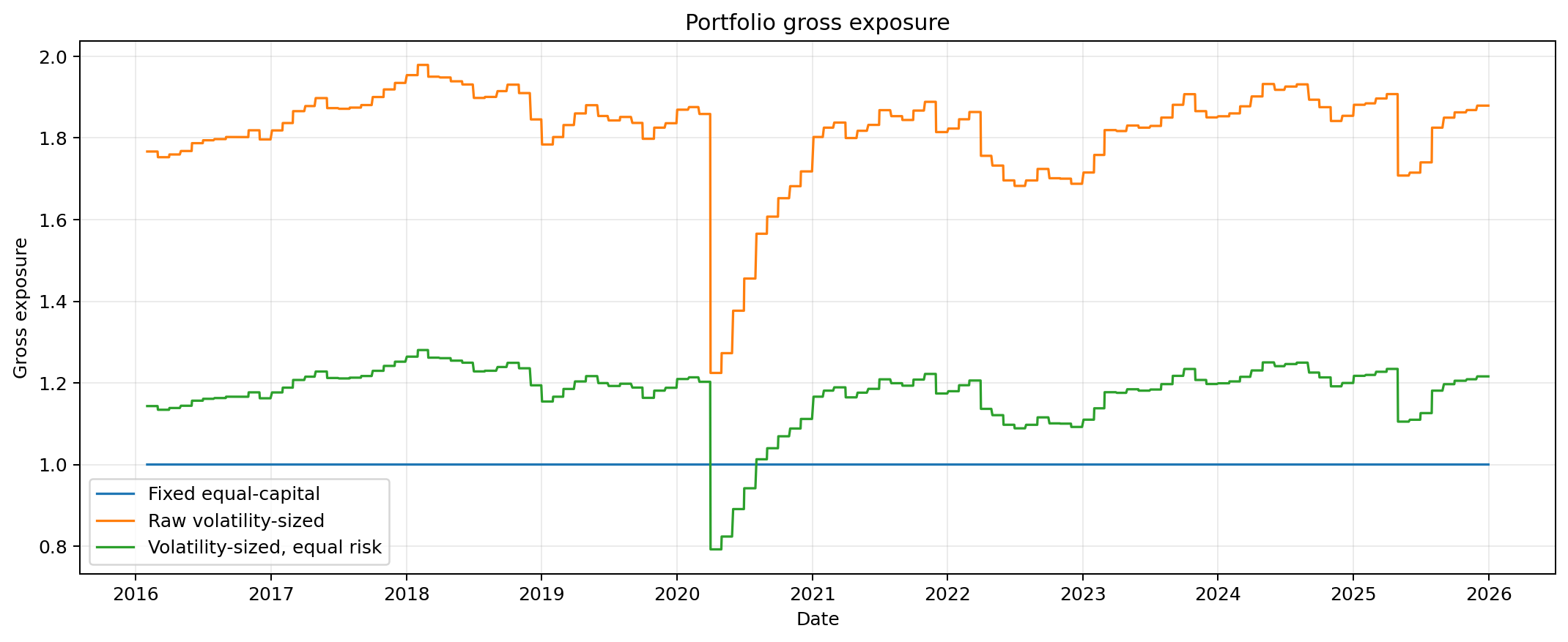
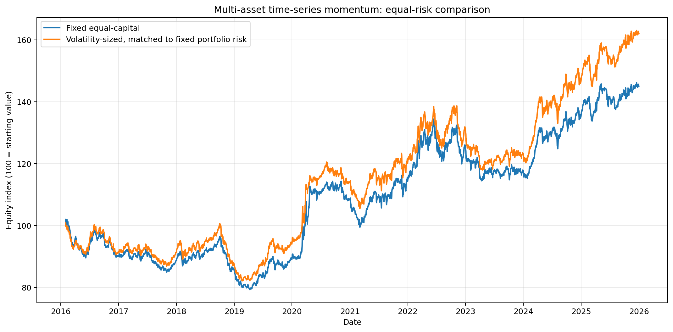
To make the comparison fairer, the volatility-sized return stream was scaled down so it had the same full-sample realized annualized volatility as the fixed portfolio. This is an after-the-fact analytical control, not a live trading rule.
After this adjustment, both portfolios had about 9.72% annualized realized volatility.
| Metric | Fixed equal-capital | Volatility-sized, equal risk |
|---|---|---|
| CAGR | 3.71% | 4.94% |
| Annualized volatility | 9.72% | 9.72% |
| Sharpe ratio (0% cash) | 0.44 | 0.55 |
| Maximum drawdown | −22.31% | −18.59% |
| Ending equity index | 145.1 | 162.0 |
| Average gross exposure | 1.00× | 1.17× |
| Maximum gross exposure | 1.00× | 1.28× |
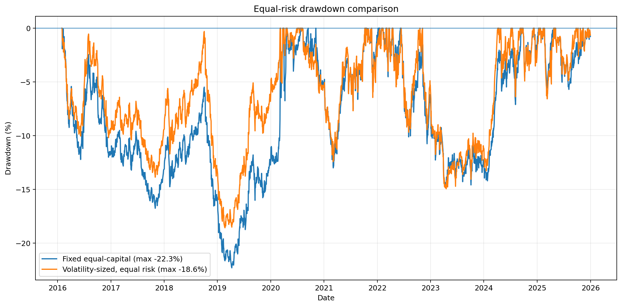
At equal realized portfolio risk, the dynamically sized version produced a higher CAGR (compound annual growth rate), a higher Sharpe ratio (return per unit of risk), a shallower maximum drawdown, and a higher ending equity index. Three reasons it helped in this sample: high-volatility assets were prevented from dominating the whole portfolio, exposure adapted through time as each asset's estimated volatility changed, and the sleeves were not perfectly correlated, so risk could spread across different markets.
What this does and does not prove
The example shows volatility sizing can add value in a multi-asset trend portfolio, especially once the comparison is made at equal realized risk. It does not prove that volatility management always improves performance. The research is mixed in an important way: Moreira and Muir (2017) found strong benefits to volatility-managed portfolios, while Cederburg, O'Doherty, Wang and Yan (2020) found that volatility management did not produce universally reliable out-of-sample improvements across a broad range of equity strategies. Volatility persistence alone is not enough; signal quality, transaction costs, implementation, leverage caps and the relationship between expected returns and volatility all matter.
Daily direction is difficult to forecast from yesterday's return, but the size of market movement is meaningfully persistent. That makes volatility useful for sizing and risk allocation, not as a direct prediction of up versus down.
Why this is relevant to prop firm trading
Prop firm challenges are won or lost on risk control, not on being right more often. The core idea here, that a fixed number of contracts is not a fixed amount of risk, is exactly what trips up evaluations: the same size that is safe in a calm session can breach a daily loss limit or a trailing drawdown in a volatile one. Scaling size to current volatility is one way traders keep risk steady across conditions. None of this is a recommendation to trade any particular way; whatever sizing rule you use, the honest step before paying for a challenge is to test it. Turn a risk percentage into a real trade with the position size calculator, and estimate how a given risk level holds up against a firm's rules with the pass rate simulator.
Methodology summary
| Component | Specification |
|---|---|
| Markets | IVV, TLT, GLD, USO and DBA |
| Asset classes | US equities, Treasury bonds, gold, oil and agriculture |
| Data source | PortBench Market Base Dataset |
| Source period | 2 January 2015–31 December 2025 |
| Active strategy period | 1 February 2016–31 December 2025 |
| Directional signal | Sign of the previous 12-month return |
| Holding period | One month |
| Fixed portfolio | Equal 20% absolute allocation per asset |
| Volatility estimator | Exponentially weighted daily volatility |
| EWMA centre of mass | 60 trading days |
| Standalone volatility target | 40% annualized |
| Per-asset multiplier cap | 2× |
| Rebalancing | Monthly |
| Equal-risk control | Ex-post scaling to 9.72% annualized realized volatility |
| Trading costs | Excluded |
Size your risk, then test your odds
Whatever sizing rule you use, the last step before a prop challenge is to check the numbers. Turn a risk percentage into a real position, then estimate your odds of passing against a firm's rules.
Open the position size calculator →See your estimated pass rate against each firm.
Open the pass rate simulator →Frequently asked questions
Can you predict market volatility?
Not perfectly, but volatility is far more forecastable than daily direction. Large moves tend to cluster near other large moves and calm periods tend to persist, a well-documented effect called volatility clustering. That persistence is what makes volatility useful for sizing and risk allocation, not for predicting up versus down.
What is volatility clustering?
The tendency for the size of price moves to persist: volatile days tend to be followed by volatile days, and calm by calm. It is one of the most established empirical features of financial markets, and it is why the magnitude of returns carries more short-term information than the direction.
What is volatility-based position sizing?
A rule that sets position size from estimated risk rather than conviction. A basic inverse-volatility rule multiplies your position by target volatility divided by estimated volatility, so a position shrinks when volatility rises and can grow when it falls, usually subject to a leverage cap.
Does volatility targeting always improve returns?
No. In the example here it improved the return-to-risk trade-off once both portfolios were matched to the same realized risk. But the research literature is mixed: some studies find clear benefits and others find no reliable out-of-sample improvement. Signal quality, costs, leverage caps and implementation all matter.
What is time-series momentum?
A strategy that goes long an instrument if its own recent return (here the trailing 12 months) was positive and short if it was negative, then holds for a set period. It was documented by Moskowitz, Ooi and Pedersen (2012). This article uses it only as a transparent framework to demonstrate sizing, not as a recommendation.
Is this a trading strategy I should use?
No. This is an educational review of an idea and a single historical example with costs excluded. It is not advice to trade time-series momentum, use leverage, or size any specific way. Any approach needs to be tested on your own data, instruments and rules before it means anything.
References
- Andersen, T. G., & Bollerslev, T. (1997). Intraday periodicity and volatility persistence in financial markets. Journal of Empirical Finance, 4(2–3), 115–158.
- Andersen, T. G., & Bollerslev, T. (1998). Deutsche Mark–Dollar volatility. The Journal of Finance, 53(1), 219–265.
- Andersen, T. G., Bollerslev, T., Diebold, F. X., & Labys, P. (2003). Modeling and forecasting realized volatility. Econometrica, 71(2), 579–625.
- Baltussen, G., van Bekkum, S., & Da, Z. (2019). Indexing and stock market serial dependence around the world. Journal of Financial Economics, 132(1), 26–48.
- Cederburg, S., O'Doherty, M. S., Wang, F., & Yan, X. (2020). On the performance of volatility-managed portfolios. Journal of Financial Economics, 138(1), 95–117.
- Cont, R. (2001). Empirical properties of asset returns: Stylized facts and statistical issues. Quantitative Finance, 1(2), 223–236.
- Engle, R. F. (2004). Risk and volatility: Econometric models and financial practice. American Economic Review, 94(3), 405–420.
- Moreira, A., & Muir, T. (2017). Volatility-managed portfolios. The Journal of Finance, 72(4), 1611–1644.
- Moskowitz, T. J., Ooi, Y. H., & Pedersen, L. H. (2012). Time series momentum. Journal of Financial Economics, 104(2), 228–250.
- Zhao, Y., Chen, S., & Su, N. (2026). PortBench: A correlation-aware, full-pipeline benchmark for LLM-driven portfolio management. arXiv.