 DanFin
Why ICT and SMC Are Not a Viable Strategy on Their Own
In short
- ICT and SMC are usually taught as a vocabulary of chart concepts, not as one standardised strategy with fixed rules.
- A payout proves a profitable outcome happened. It does not isolate skill from variance, selection bias or favourable conditions.
- Flexible concepts are easy to reinterpret after the result and easy to overfit in a backtest.
- Order flow is a real market variable, but that does not validate every retail order-flow interpretation.
- An ICT or SMC idea becomes a viable research candidate only once its rules are fixed in advance and survive unseen data, costs and statistical uncertainty.
Payouts, funded accounts and convincing chart explanations can all be genuine. None of them, by themselves, establishes that the method behind them has positive expectancy. This is an evidence-led look at why, and at what it would actually take to show an ICT or SMC idea works.
- The claim being evaluated
- A framework is not a strategy
- Why falsifiability matters
- An edge is a number
- Why payouts don't prove skill
- The prop-firm probability example
- Backtest overfitting
- Why a short track record is weak
- What retail research finds
- Order flow is real, but...
- The institutional-footprint story
- Why lower timeframes are harder
- Making the concepts testable
- FAQ
Claim your spot on the waitlist
I am releasing one of my trading strategies shortly. Join the waitlist and receive a discount at launch.
Claim your spot →1. The claim being evaluated
The strongest defensible criticism of ICT (Inner Circle Trader), SMC (Smart Money Concepts) and retail order-flow trading is not that every trader using them must lose. That would be too absolute, and the public evidence does not justify it. The more precise criticism is this:
As commonly taught, ICT and SMC do not by themselves constitute a viable trading strategy. They are a flexible interpretive framework that still has to be converted into fixed, falsifiable and independently validated rules.
A trader may use the words order block, fair-value gap, liquidity sweep, market-structure shift, premium and discount, higher-timeframe bias and kill zone. Those labels can help organise a chart. They do not automatically tell us whether the resulting decisions have positive expectancy after costs. And there is no single universally accepted "ICT strategy" to test: different educators define the same concepts differently, combine them in different orders, and add different exceptions. That shifts the burden of proof onto the specific rule set being traded.
2. A framework is not yet a strategy
A viable strategy must map information available at time t into an action that can be evaluated after time t. At minimum it needs to specify the market and data source, the timeframe and session, the exact setup conditions, the entry trigger, the condition that invalidates the setup, the stop, exit and time-out rules, the position-sizing rule, all permitted exceptions, and the assumed spread, commissions and slippage.
Compare that with a basic moving-average rule: "go long at the next open when the 10-day average crosses above the 30-day average; exit when it crosses below." That rule may or may not be profitable, but it is objective. Brock, Lakonishok and LeBaron (1992) could test moving-average and trading-range-break rules precisely because they had a reproducible form, and Sullivan, Timmermann and White (1999) could then ask whether the strongest historical result survived a correction for data snooping and a later out-of-sample period.
Many ICT and SMC explanations are less constrained. Two traders can mark different order blocks on the same chart: one using the candle body, another the full wick, another the final down candle before displacement, another a nested block from a lower timeframe. That flexibility is not a small technical problem. It creates a very large hidden search space, where every additional choice is another variant that could be selected after seeing which version worked best.
| Concept | Common ambiguity | What a testable rule must specify |
|---|---|---|
| Order block | Which candle, body or wick, freshness, mitigation, timeframe | Exact candle pattern, price bounds, expiry and invalidation |
| Fair-value gap | Minimum size, wick/body treatment, partial fill, nested gaps | Three-candle formula, minimum threshold and fill rule |
| Liquidity sweep | Which high or low counts and how far price must trade through it | Reference level, penetration threshold and closing requirement |
| Market-structure shift | Internal versus external structure; wick versus close | Pivot algorithm, break threshold and confirmation timing |
| Higher-timeframe bias | Daily, four-hour or weekly; trend, range or narrative | One deterministic calculation available before entry |
3. Why falsifiability matters
A useful trading hypothesis must be able to fail. If no possible result can count against it, the framework can explain history but cannot establish predictive power. After a losing trade, an ICT-style explanation can often be changed: the wrong order block was selected, the block was only a mitigation block, the higher-timeframe bias had priority, external liquidity had not yet been taken, the entry was outside the correct kill zone, or the apparent structure shift was only internal. Any one of those distinctions could be useful if it was defined before the trade. The problem is when it only becomes clear after the loss.
Discretion does not make testing impossible; it changes what must be recorded. A discretionary trader can time-stamp the complete pre-trade thesis, the marked levels, screenshots, permitted actions and invalidation before the outcome is known. Independent reviewers can then measure whether different trained users apply the framework consistently. Without that record, hindsight silently improves every historical explanation, which is the core mechanism behind survivorship bias in trading.
4. An edge is a number
A strategy has an economic edge when its expected profit stays positive after costs. A simple trade-level expression is:
where p is the win probability, W the average gross win, L the average gross loss, and C the average cost of spread, commissions and slippage. Suppose a strategy wins 45% of trades, makes $220 on the average winner, loses $160 on the average loser and pays $14 in costs:
The setup can still produce impressive winning streaks and profitable months, yet its estimated average is negative. A genuinely positive strategy can also suffer a long drawdown. That is why individual outcomes do not identify expectancy. Even a positive sample estimate is not enough, because it has uncertainty: if 80 trades average +$9 with a standard deviation of $190, the standard error is about $190 ÷ √80 ≈ $21. A +$9 average is small relative to that, and does not reliably separate a real edge from zero. This is the same relationship between win rate, reward-to-risk and expectancy.
5. Why payouts do not prove skill
A payout is evidence that a trader followed one profitable path. It is not evidence that the underlying distribution had positive drift. Imagine 2,000 traders, each taking 200 independent trades, every trade a 50% chance of +$100 and 50% chance of −$100. The expectancy before costs is exactly $0. No trader has an edge, yet the ending results are widely dispersed: several curves look disciplined and profitable, others disastrous. Selecting a winning curve afterward makes random performance look like skill.
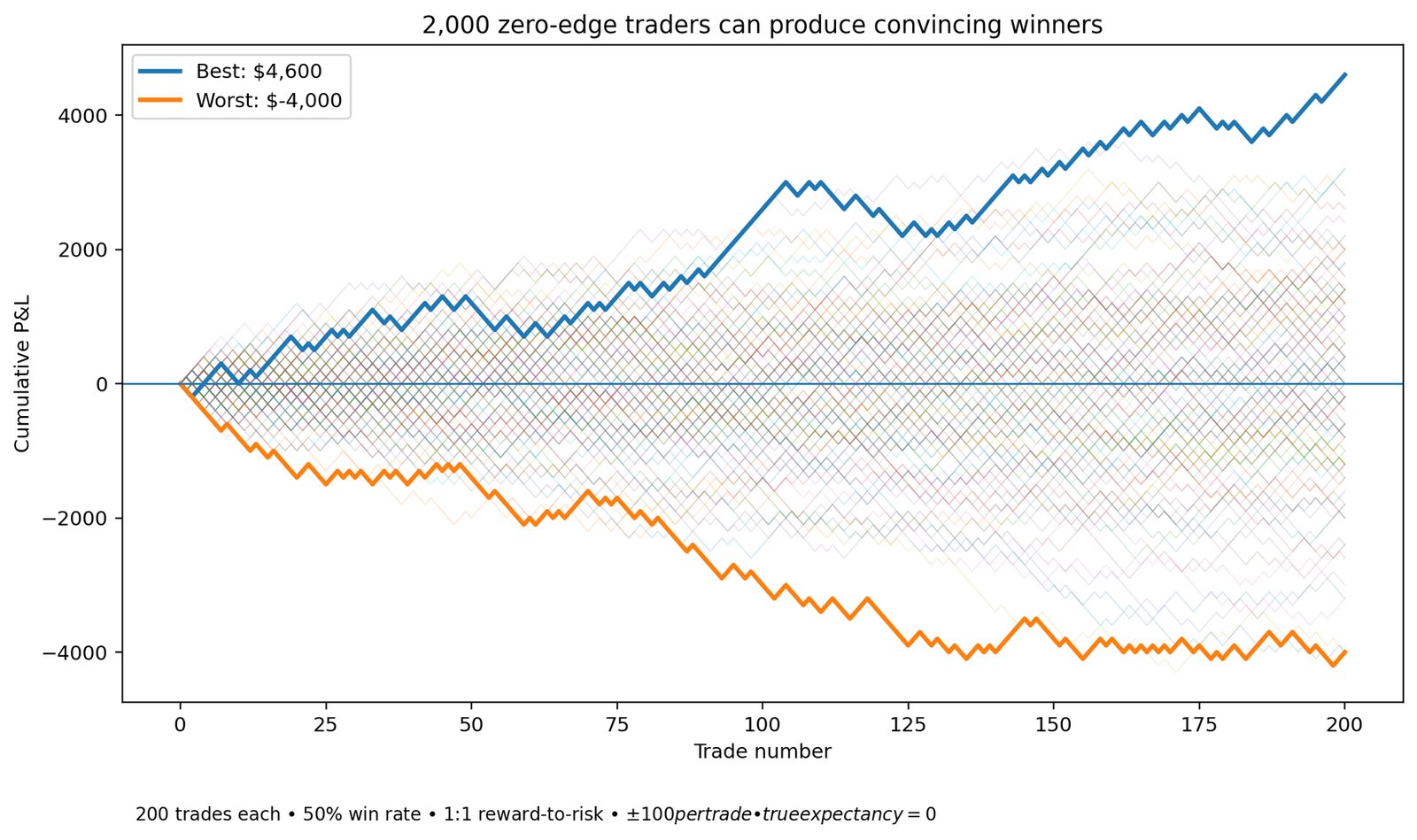
On social media this is more persuasive because the sample is hidden. The trader with the profitable curve posts it; the failed accounts go quiet. It is a combination of variance (different outcomes from the same process), survivorship bias (failed attempts removed from view) and selection bias (attention focused on the best result after it is known). The winning payout may be completely authentic. The inference from payout to edge is the weak step.
6. The prop-firm probability example
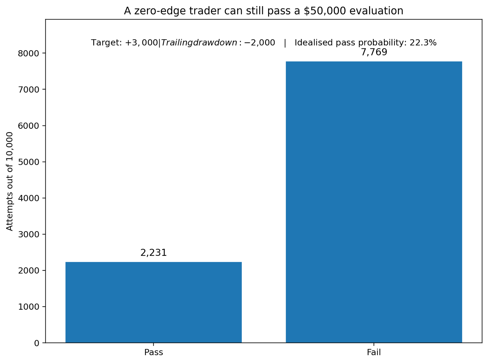
Prop-firm evaluations make the outcome-versus-edge distinction especially clear. A challenge asks the trader to reach a profit target before violating a loss limit, which is a barrier-hitting problem. In an idealised continuous zero-drift model with a trailing drawdown of size d, the running maximum reached before the first drawdown is exponentially distributed (Landriault, Li and Zhang, 2015), and the probability of reaching target T before the trailing drawdown is:
Applied to 10,000 independent attempts, that is about 2,231 passes generated by a process with zero drift.
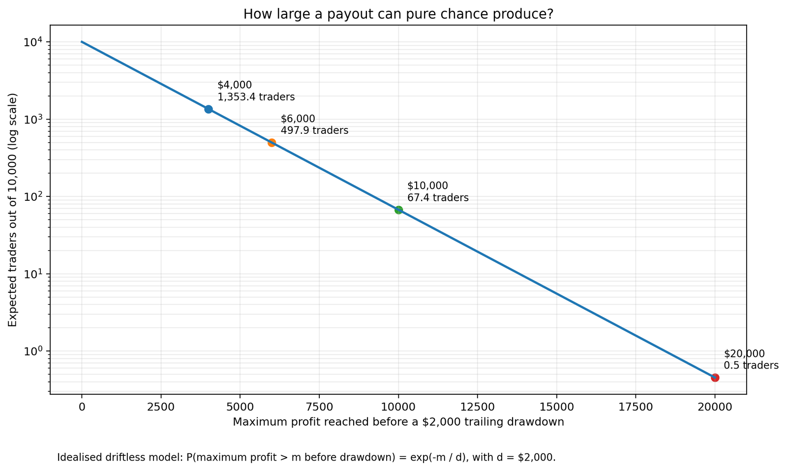
The same result explains why large payouts do not logically require positive drift. The probability that the running maximum exceeds amount m before a $2,000 trailing drawdown is exp(−m / $2,000), so among 10,000 zero-edge attempts the expected number reaching each level is:
| Maximum profit reached first | Probability | Expected out of 10,000 |
|---|---|---|
| More than $4,000 | 13.53% | 1,353 |
| More than $6,000 | 4.98% | 498 |
| More than $10,000 | 0.67% | 67 |
| More than $20,000 | 0.0045% | 0.45 |
7. Backtest overfitting and multiple testing
"I backtested it" is not the end of the discussion. A backtest becomes unreliable when the same data are used repeatedly to invent, modify and select the rules. White (2000) calls this data snooping: try enough models and satisfactory results arise by chance. ICT and SMC frameworks create an especially large search space, because the researcher can vary the structure timeframe, the order-block definition, the gap threshold, the liquidity level, the session, the confirmation trigger, the stop, the reward target, the assets and period, and which "low-quality" setups are removed after inspection.
Even assuming independent tests, the probability of at least one false positive at a 5% level is 1 − (1 − 0.05)N:
| Number of tested variants | Chance of at least one false positive |
|---|---|
| 1 | 5.0% |
| 20 | 64.2% |
| 100 | 99.4% |
Real searches are correlated, so this is not an exact correction, but it shows the direction: picking the best of many attempts makes the ordinary threshold too permissive. Harvey, Liu and Zhu (2016) make the same point in asset pricing, where the conventional t-statistic near 2 became inadequate after hundreds of factors had been tried.
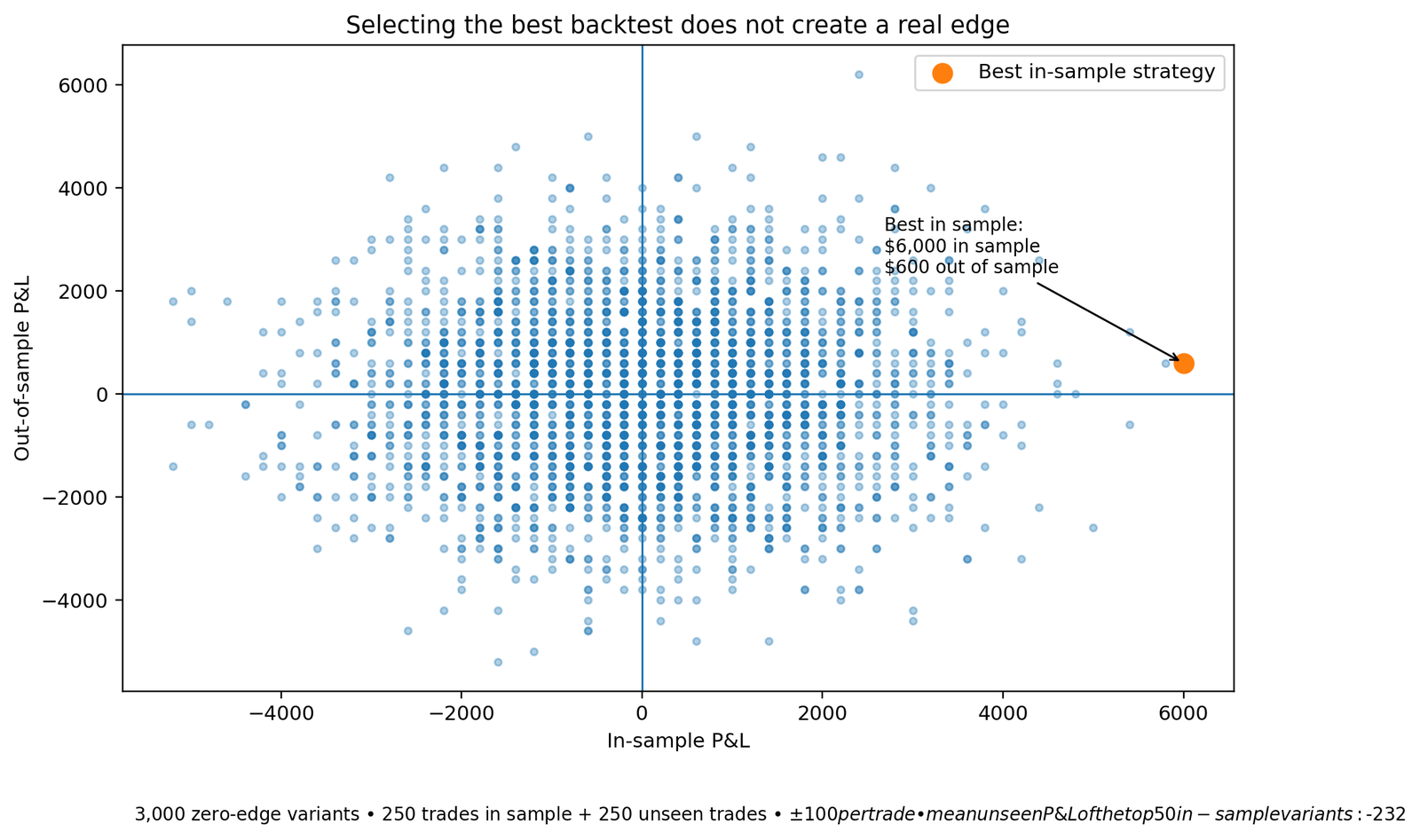
Bailey, Borwein, Lopez de Prado and Zhu (2017) formalise the probability of backtest overfitting: the best in-sample configuration can be the one most favoured by noise. Sullivan et al. (1999) found the best technical rules looked far less convincing after the search and a later period were accounted for. Objective rules face this problem; flexible discretionary rules face it with even more degrees of freedom. If you are working from research, how to read the research behind a strategy and how to backtest properly cover the guards.
8. Why a short track record is weak evidence
A Sharpe ratio, win rate or average return is an estimate, not a fixed property revealed perfectly by a small sample. Lo (2002) shows Sharpe inference depends on the return distribution and serial correlation. Under an ideal independent-normal approximation, the statistical strength of an annualised Sharpe grows roughly with the square root of the number of years:
So a true Sharpe of 0.5 needs about 16 years to reach t = 2, and about 36 years for t = 3; a true Sharpe of 1.0 needs about 4 years for t = 2 under the same assumptions.
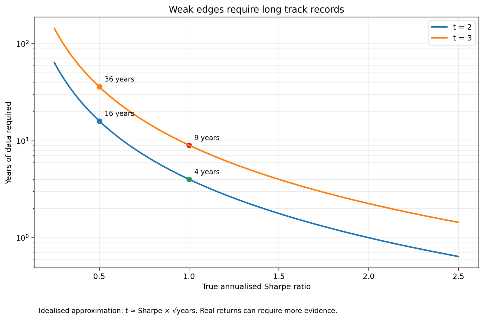
This does not mean every useful strategy needs decades of live data; researchers can add independent observations across instruments and regimes if the design accounts for correlation. But it shows why a few months of payouts or one favourable regime are weak evidence for a modest edge, and why an extreme short-sample Sharpe is exactly what you expect when many traders, markets and parameters are observed and only the best are shown.
9. What retail-trader research actually finds
Large empirical studies do not support the idea that retail day trading is broadly and reliably profitable after costs. They also do not support the absolute claim that no retail trader can have skill. Barber, Lee, Liu and Odean (2014) studied Taiwanese day traders from 1992 to 2006 and found a small group with persistent skill, but fewer than 1% could predictably earn positive abnormal returns net of fees, and most apparent success was luck. Chague, De-Losso and Giovannetti (2020) followed people who day-traded Brazilian index futures for at least 300 days: 97% lost money, only 0.4% earned more than a bank teller's daily wage, and there was no evidence performance improved with experience.
These studies concern particular markets and populations and do not directly test ICT or SMC. Their relevance is methodological: visible winners cannot be interpreted without the full population, costs and persistence.
10. Order flow is real, but that is a different claim
Criticising retail order-flow claims does not require denying market microstructure. Order flow is real: limit-order books, market orders, cancellations, depth and queue position influence short-horizon prices. Cont, Kukanov and Stoikov (2014) found a strong relationship between order-flow imbalance at the best bid and ask and contemporaneous price changes, with sensitivity inversely related to depth. But three distinctions matter: a contemporaneous relation is not automatically a forecast; forecasting is not the same as execution profit once you subtract spread, commissions, slippage, latency and adverse selection; and market data differ by venue, so futures, fragmented equities, spot FX and CFD feeds do not reveal the same information. The question is not whether order flow exists, but whether one precisely defined transformation of it predicts future returns after costs.
11. The institutional-footprint story is too simple
A recurring ICT and SMC narrative is that institutions leave obvious footprints a retail trader can read on candlesticks. The kernel of truth is that large orders can move prices and cannot always be executed instantly. The oversimplification is assuming one candle pattern reliably reveals the origin, intention and remaining size of that activity. The Bank for International Settlements' report on FX execution algorithms describes a far more complex process: large parent orders are sliced into many child orders, routed across fragmented venues, internalised, executed in dark liquidity and scheduled through algorithms such as VWAP or TWAP, specifically to manage impact and information leakage. So a retail candlestick is the aggregate of many participants, venues and motives, and marking the final down candle before a rally does not identify an institutional position. The label "institutional" adds a story, not evidence.
12. Why lower timeframes raise the evidentiary bar
Many ICT, SMC and order-flow strategies operate on very short horizons. In a simple diffusion model, expected drift over horizon h scales with h while volatility scales with √h, so the drift-to-volatility ratio is (μ / σ) × √h. As the horizon shrinks, long-run drift becomes tiny relative to ordinary variation, so a one-minute trader cannot lean on the market's long-term upward drift; the edge must come from a specific conditional pattern.
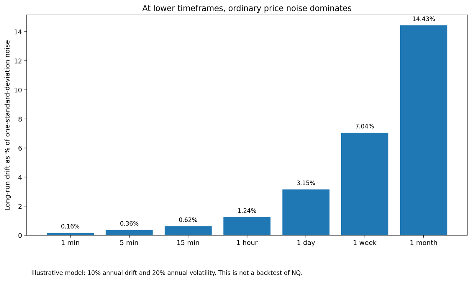
Costs also matter more as profit per trade shrinks. A setup that appears to earn $8 per trade before costs can be negative after a $4 commission, $2 spread and $5 average slippage, and event-driven periods widen spreads exactly when the chart looks most attractive. The conclusion is not that low-timeframe trading is impossible; it is that the evidentiary standard should be higher, not lower.
13. How to turn ICT or SMC concepts into a testable strategy
A trader who wants to move from narrative to evidence does not need to abandon every concept. The concepts have to be operationalised.
Step 1: freeze the information set. Specify exactly what data are allowed at the moment of decision, so future swings and session extremes cannot leak into the choice. Step 2: define every concept numerically. For example:
| Component | Example of an objective specification |
|---|---|
| Liquidity sweep | Price trades at least 0.10 ATR above the previous session high and closes back below it within two five-minute bars. |
| Market-structure shift | A five-minute close below the most recent confirmed swing low, where a swing low requires two higher lows on each side. |
| Fair-value gap | For three consecutive bars, the third bar's high is below the first bar's low by at least 0.05 ATR. |
| Entry | A limit order placed at the midpoint of the first qualifying gap, valid for three bars. |
| Invalidation | A stop one tick above the sweep high; the order is cancelled if not filled within three bars. |
| Exit | A profit target at 2R, a stop at -1R, or a time-based exit at 15:55 New York time. |
These are examples of how to specify a rule precisely enough to test, not recommended parameters or a suggested setup.
Step 3: register the rule before the final test. Split the data into development, validation and final-test periods, record the rule before viewing the final test, and use that period once. Step 4: include realistic implementation, the actual instrument, tick size, commissions, spread, order type, fills and slippage. Step 5: report the distribution, not only the average, including the number of trades, the confidence interval around expectancy, the drawdown, results by year and regime, parameter sensitivity, and every tested variant, not only the winner. Step 6: test whether discretion is reproducible by giving the same unseen charts to several trained users and measuring agreement. Step 7: keep a prospective record, time-stamping setups before entry and preserving rejected setups too.
Persuasive evidence would look like a public, fixed rule set; a large unseen sample; positive net expectancy with uncertainty reported; reasonable stability across periods and nearby parameters; realistic fills and costs; a prospective record that cannot be rewritten after the result; and independent replication by people other than the creator.
Conclusion
ICT, SMC and retail order-flow trading are persuasive partly because they make random market movement look intentional after the fact. Every rally links to demand, every reversal to liquidity, every failed setup to a higher-order narrative. That explanatory richness is exactly why the frameworks require stricter testing: a method with many flexible labels can explain almost any completed chart, and predictive value begins only when the interpretation is fixed before the outcome.
Payouts prove that an outcome happened. A viable strategy requires evidence that the outcome was generated by repeatable positive expectancy rather than chance, selection and hindsight.
As commonly taught, ICT and SMC do not yet meet that standard. They are frameworks from which a strategy might be constructed, not evidence that a viable strategy already exists.
A pass is not proof of an edge
As the maths here shows, even a zero-edge run can hit a target before a drawdown. Before you trust any method, estimate your real odds: enter your win rate, reward-to-risk and risk per trade and see how a strategy holds up against a firm's rules.
Open the pass rate simulator →New to prop firms? Start with the fundamentals.
Read the beginner's guide →Frequently asked questions
Does this prove every ICT or SMC trader loses money?
No. It shows that ICT and SMC, as commonly taught, are flexible descriptive frameworks rather than one standardized strategy with a demonstrated edge. A trader could potentially turn parts of the framework into objective rules and validate those rules, but the labels themselves do not prove profitability.
Can a profitable payout still be caused by luck?
Yes. A payout confirms that a profitable path occurred. It does not by itself identify whether the path came from skill, positive expectancy, favourable conditions, selection bias, or ordinary variance.
Is order flow real?
Yes. Research documents relationships between order-flow imbalance and short-horizon price changes. That is different from proving that a retail DOM, footprint chart or candlestick interpretation delivers a profitable forecast after spread, commissions, slippage, latency and adverse selection.
How can an ICT or SMC idea become testable?
Define every condition before the trade: market, timeframe, session, setup, entry, invalidation, exit, position size, costs and exceptions. Freeze those rules, test them on unseen data, report the uncertainty, and keep a live time-stamped record.
Does passing a prop-firm evaluation prove a strategy has an edge?
No. A pass is one path through a target-and-drawdown problem. The probability depends on the strategy, rules, risk per trade, daily limits, trailing mechanics, costs and time horizon. Even a zero-drift process can reach a profit barrier before a drawdown barrier in an idealised model.
Methodology and modelling notes
- Zero-edge equity curves: 2,000 simulated traders; 200 independent trades each; 50% chance of +$100 and 50% of -$100; no costs.
- Prop-firm barrier example: driftless continuous Brownian motion; +$3,000 target; -$2,000 drawdown from the running maximum; no time limit, costs, jumps or discrete-trade effects.
- Payout-tail example: the same Brownian assumptions, using the exponential distribution of the running maximum before a fixed drawdown.
- Backtest-overfitting graph: 3,000 independent zero-edge variants; 250 trades in sample and 250 unseen out of sample.
- Sharpe graph: the simplified independent-normal approximation t ≈ Sharpe × √years, used for intuition rather than exact inference.
- Signal-to-noise graph: a simple diffusion illustration using 10% annual drift and 20% annual volatility.
These examples isolate one statistical mechanism at a time. Real returns can show skewness, fat tails, serial dependence, volatility clustering, changing regimes, correlated positions and execution effects.
References
Bailey, D. H., Borwein, J. M., Lopez de Prado, M., & Zhu, Q. J. (2017). The probability of backtest overfitting. Journal of Computational Finance, 20(4), 39–69.
Bank for International Settlements, Markets Committee. (2020). FX execution algorithms and market functioning. Bank for International Settlements.
Barber, B. M., Lee, Y.-T., Liu, Y.-J., & Odean, T. (2014). The cross-section of speculator skill: Evidence from day trading. Journal of Financial Markets, 18, 1–24.
Brock, W., Lakonishok, J., & LeBaron, B. (1992). Simple technical trading rules and the stochastic properties of stock returns. The Journal of Finance, 47(5), 1731–1764.
Chague, F., De-Losso, R., & Giovannetti, B. (2020). Day trading for a living? (FGV EESP Working Paper No. 525).
Cont, R., Kukanov, A., & Stoikov, S. (2014). The price impact of order book events. Journal of Financial Econometrics, 12(1), 47–88.
Harvey, C. R., Liu, Y., & Zhu, H. (2016). ... and the cross-section of expected returns. The Review of Financial Studies, 29(1), 5–68.
Landriault, D., Li, B., & Zhang, H. (2015). On the frequency of drawdowns for Brownian motion processes. Journal of Applied Probability, 52(1), 191–208.
Lo, A. W. (2002). The statistics of Sharpe ratios. Financial Analysts Journal, 58(4), 36–52.
Sullivan, R., Timmermann, A., & White, H. (1999). Data-snooping, technical trading rule performance, and the bootstrap. The Journal of Finance, 54(5), 1647–1691.
White, H. (2000). A reality check for data snooping. Econometrica, 68(5), 1097–1126.