 DanFin
Hidden Markov Models in Trading: Detecting Market Regimes Without Pretending to Predict the Future
In short
- Markets move through persistent "regimes", stretches of calm or turbulent, favourable or adverse conditions. A hidden Markov model estimates which one you are in from returns and volatility.
- It is not a crash predictor. It confirms a shift only after enough evidence arrives, so its real job is adjusting risk, not calling direction.
- The 2024 Princeton study found a "statistical jump model" gave steadier, lower-turnover signals than a plain HMM, with lower drawdowns and better risk-adjusted returns in three equity-index tests.
- For prop firms this is the useful part: the model targets when losses are likely to cluster, which is exactly what breaches a daily or trailing loss limit.
- Used as a risk filter rather than an entry signal, it can cut exposure before a bad streak reaches a hard barrier, and make pass-rate simulations more realistic.
Financial markets do not behave as one steady, predictable process. A strategy can meet months of quiet, directional price action and then suddenly face bigger gaps, wider ranges, stronger correlations and clustered losses. Quants call these persistent statistical environments market regimes, and the practical question a regime model asks is not "what happens next?" but "what kind of market are we in right now?"
A hidden Markov model, or HMM, is one of the standard tools for answering that. It assumes an unobserved state, calm or turbulent, favourable or adverse, drives the data we can see, and since the state is hidden, the model works out the probability of each one from observations such as returns and volatility. Crucially, an HMM does not spot a crash before everyone else. In live use it usually needs evidence that conditions have already changed, so its real value is adaptive risk management: cut exposure, switch strategy, or revise your assumptions once a lasting change looks credible. That is a natural fit for prop-firm trading, where staying under the loss limits matters more than predicting the next candle.
Claim your spot on the waitlist
I am releasing one of my trading strategies shortly. Join the waitlist and receive a discount at launch.
Claim your spot →What is a market regime?
A regime is an extended period in which market behaviour is relatively homogeneous. The definition depends on the problem. A long-only equity investor may distinguish bull and bear markets; a volatility trader may distinguish compressed and turbulent conditions; a day-trading system may instead care about whether its own expectancy, slippage and adverse excursion are behaving normally.
- Return regime: positive versus negative average returns.
- Volatility regime: calm versus turbulent price movement.
- Correlation regime: diversified versus highly synchronised markets.
- Strategy regime: normal performance versus clustered underperformance.
Regime models are useful because abrupt changes can persist. Hamilton's foundational regime-switching work treated changes in the parameters of an autoregressive process as the outcome of a discrete-state Markov process. Later financial applications used related models to represent volatility clustering, fat-tailed returns and time-varying investment opportunities (Hamilton, 1989; Ang & Timmermann, 2012).
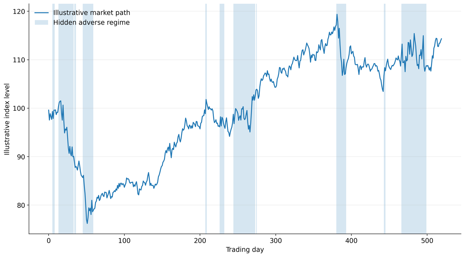
How a hidden Markov model works
An HMM has two layers. The hidden layer contains the regime, written Sₜ. The observable layer contains the data, written Xₜ. In trading, Xₜ may be a daily return, a vector of returns and volatility features, or the return stream of a strategy.
1. The hidden state follows a Markov process
The first-order Markov assumption says the probability of tomorrow's state depends on today's state, once today's state is known:
For two states, the transition matrix contains four probabilities. Large diagonal probabilities imply persistence: once the model enters a state, it expects to remain there. If pₖₖ is the probability of remaining in state k, the conventional HMM implies an expected state duration of about:
2. Each state has an observation distribution
A basic financial HMM assumes returns are normally distributed within each state, but with different means and variances:
After estimation, one state may show low volatility and a mildly positive mean, while another shows high volatility and a negative mean. The algorithm does not inherently know the words bull, bear, good or bad. The researcher assigns those interpretations after inspecting the fitted state characteristics.
3. The model estimates probabilities, not certainty
The central live quantity is the filtered probability P(Sₜ = k | X₁:ₜ), which in plain terms is the model's best current guess of which regime you are in, using only the data seen so far. A researcher can also compute smoothed states that use later observations, or reconstruct the single most likely history of states with the Viterbi algorithm.
How HMMs are used in trading
Risk overlays
The most defensible application is to change exposure when the probability of an adverse regime rises. A model may move a portfolio toward cash, reduce leverage, tighten aggregate risk, or prevent new trades. Nystrup, Madsen and Lindstrom (2018) combined HMM forecasts with dynamic portfolio optimisation and emphasised both transaction costs and delayed implementation.
Strategy selection
Different strategies rely on different market structures. Trend following needs persistent movement; mean reversion needs prices to return after deviations; short-volatility strategies are vulnerable to volatility expansion. A regime model can act as a gate that chooses which strategy is allowed to trade.
Regime-dependent position sizing
Instead of switching fully between on and off, exposure can vary with regime confidence. The model output stays separate from the entry signal: the trading strategy finds opportunities, while the regime layer determines how much risk is acceptable. Turning that into an actual trade size is what the position size calculator handles.
Regime-aware simulation
An HMM provides a transition matrix and state-conditional return distributions, which can generate simulated paths where calm and stressed periods persist. This is often more realistic than randomly shuffling trades independently, because in real markets losses and volatility tend to cluster rather than arrive at random.
Why an HMM is not a reliable turning-point predictor
A regime model faces a structural trade-off. React immediately and it will classify ordinary noise as a new regime. Demand more evidence and the signal arrives later. The model therefore confirms shifts; it does not eliminate uncertainty around the turning point.
- Noisy signals: daily returns contain little information about the latent state on their own.
- Distributional assumptions: Gaussian emissions may understate skewness and fat tails.
- State-duration assumptions: a standard HMM implies geometrically distributed durations, treating every day as having the same fixed chance of ending the current regime.
- Estimation instability: likelihood optimisation can converge to local solutions and depend on starting values.
- State instability: the economic meaning of state 1 and state 2 can drift when the model is refitted.
- Model-selection risk: the number of states, features, thresholds and training window can all be overfit.
These weaknesses do not make HMMs useless. They mean the model should be judged by its out-of-sample decision value, not by how neatly it colours a historical chart.
The statistical jump model: clustering with memory
Bemporad, Breschi, Piga and Boyd (2018) introduced a general jump-model framework for temporal data. The approach alternates between fitting model parameters and finding the sequence of active models, and the state-sequence step can be solved with dynamic programming. For regime identification, the statistical jump model can be understood as k-means-style clustering with an explicit cost for changing state:
The first term rewards assigning each observation to the closest regime centroid. The second term charges a fixed jump penalty λ whenever the state changes.
- λ = 0: the method behaves like clustering without memory.
- Small λ: the model can switch frequently.
- Large λ: only a substantial and persistent change justifies a new state.
- Excessively large λ: distinct regimes may be merged and genuine changes detected too late.
The jump model is not a jump-diffusion price model. Here, "jump" refers to switching between latent model states.
HMM versus statistical jump model
| Feature | Hidden Markov model | Statistical jump model |
|---|---|---|
| Core idea | Probabilistic latent-state model | Temporally penalised clustering / model fitting |
| Persistence | Learned through transition probabilities | Directly controlled through jump penalty |
| Output | State probabilities and decoded states | Usually a discrete optimal state sequence |
| Assumptions | Requires conditional distributions | Likelihood-free in the paper's implementation |
| Strength | Probabilistic interpretation and scenario generation | Stable signals and flexible feature design |
| Main risk | Noise, misspecification, local likelihood optima | Penalty and feature-selection sensitivity |
The 2024 Princeton study
The most relevant recent paper is Shu, Yu and Mulvey's 2024 Journal of Asset Management article, by researchers from Princeton University's Department of Operations Research and Financial Engineering. It compared a conventional HMM with a statistical jump model in a deliberately simple downside-risk strategy.
Research design
- Markets: S&P 500, DAX and Nikkei 225 total-return indices.
- Data: full history 1970–2023; out-of-sample strategy test 1990–2023.
- Allocation: 100% equity in the favourable regime and 100% risk-free asset in the unfavourable regime.
- Execution: 10-basis-point one-way transaction cost and a one-day trading delay.
- HMM: two-state Gaussian model on daily log returns with a rolling 3,000-day training window.
- Jump model: two states fitted to three exponentially weighted downside-risk and Sortino features.
- Selection: smoothing and jump-penalty hyperparameters chosen through monthly walk-forward validation.
The model centroids were re-estimated every six months over a 3,000-day window, and the penalty was updated monthly, chosen to maximise the following month's validation Sharpe ratio after costs and delay (Shu et al., 2024). The jump-model features were:
| Category | Feature | Half-life |
|---|---|---|
| Risk | Exponentially weighted downside deviation | 10 trading days |
| Return | Exponentially weighted Sortino ratio | 20 trading days |
| Return | Exponentially weighted Sortino ratio | 60 trading days |
Finding 1: the raw HMM signal was unstable
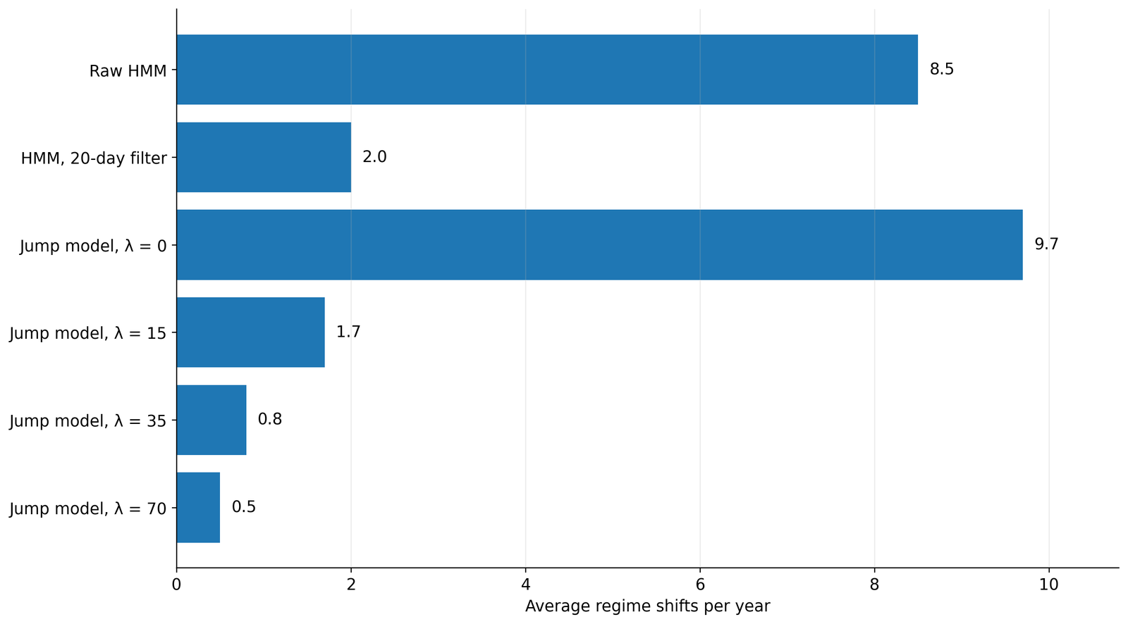
From 1982 to 2023, the unsmoothed online HMM signal switched an average of 8.5 times per year. A 20-day median filter cut this to 2.0 switches, but that smoothing creates at least about ten days of signal latency. The jump model gave more direct control over persistence: a penalty of 35 produced 0.8 shifts per year and a penalty of 70 produced 0.5.
Finding 2: downside risk improved in the equity-index backtests
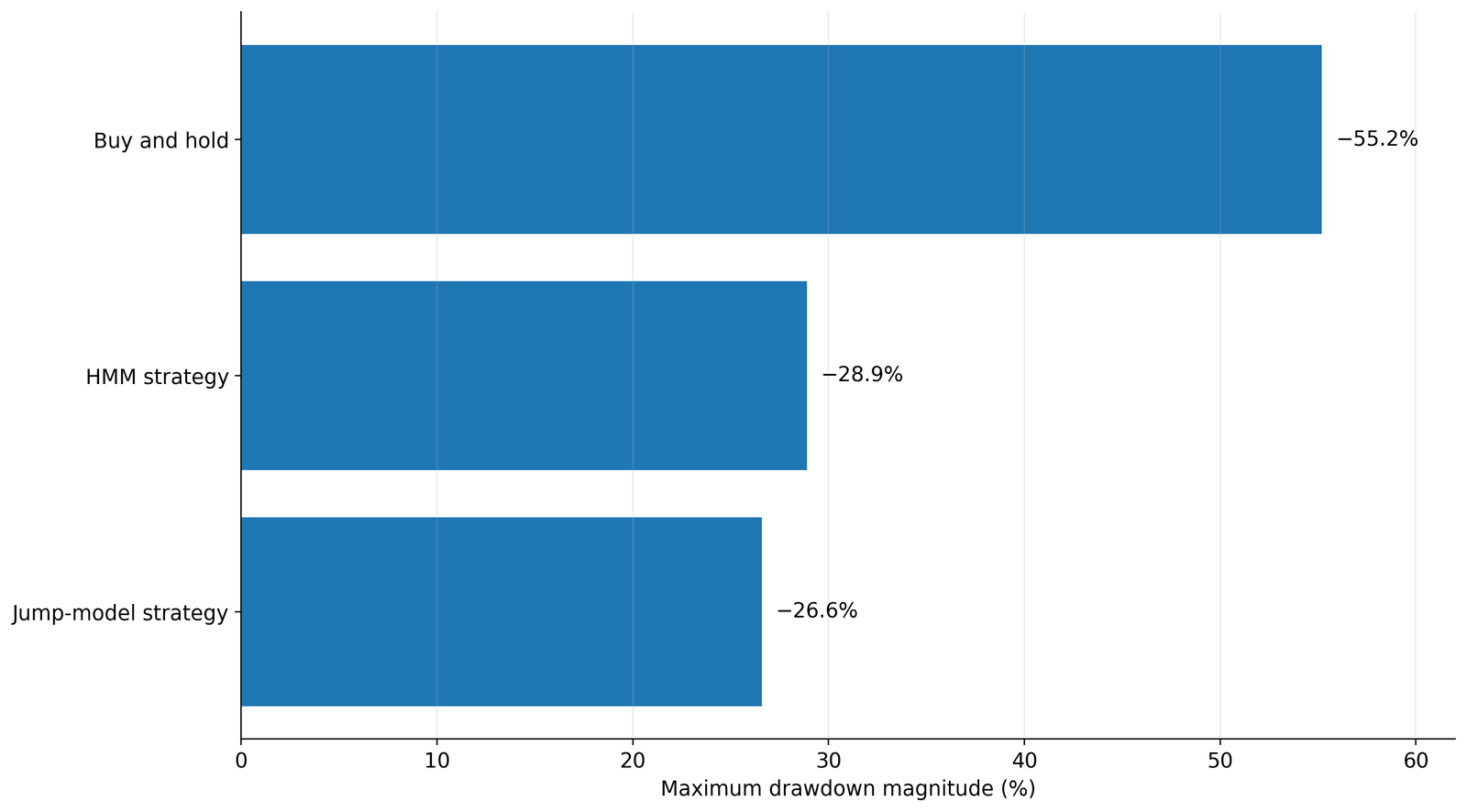
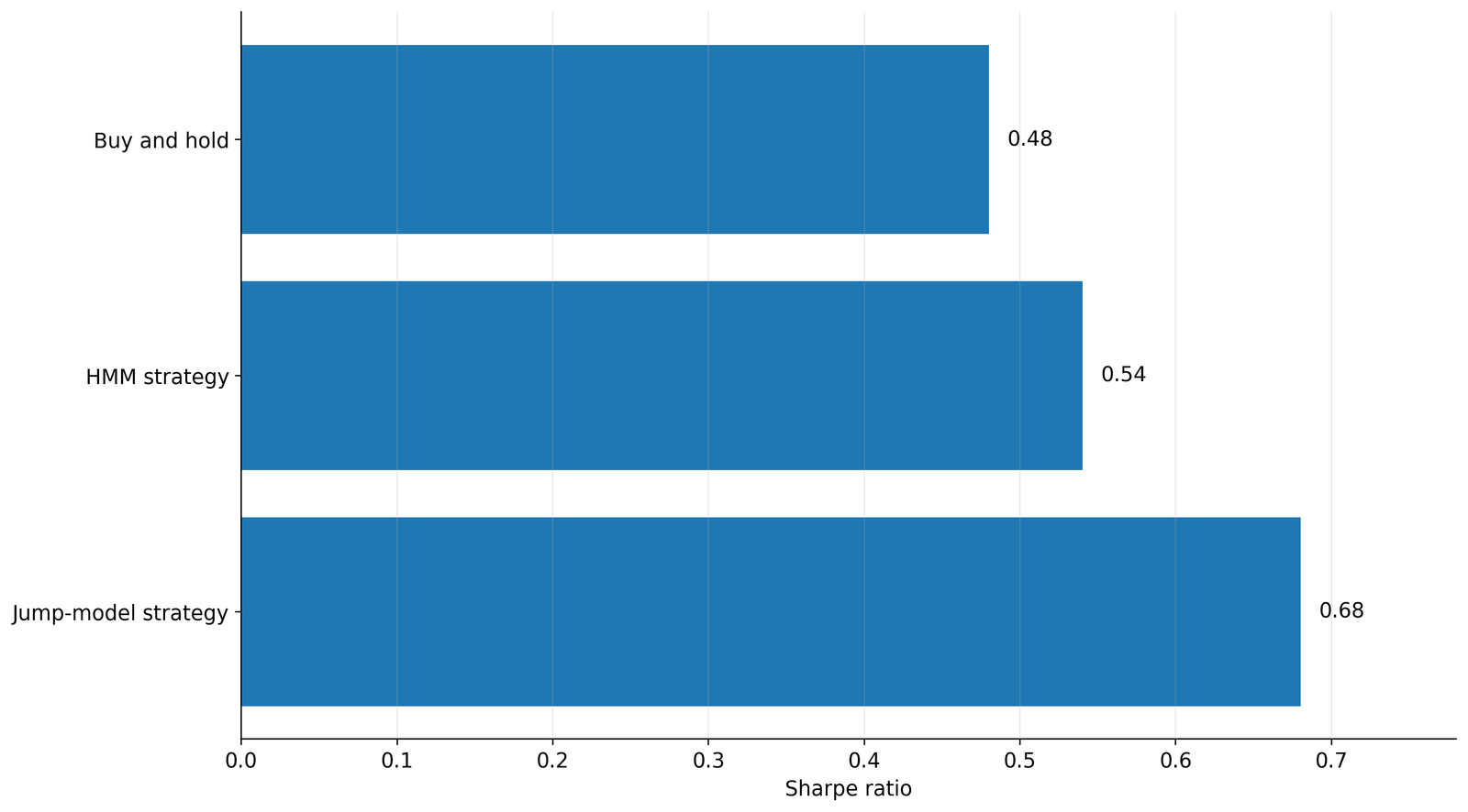
For the S&P 500, buy-and-hold produced a reported maximum drawdown of −55.2%. The HMM-guided strategy reduced it to −28.9%, and the jump-model strategy to −26.6%. The corresponding Sharpe ratios were 0.48, 0.54 and 0.68. The same broad ranking appeared for the DAX and Nikkei 225, although the exact performance differed across markets.
Finding 3: persistence improved implementation robustness
The jump-model strategy had materially lower turnover than the HMM strategy. On the S&P 500, reported annual turnover was 44% for the jump model versus 141% for the HMM. The authors also tested 1-, 5- and 10-day delays. Performance generally weakened with longer delays, especially outside the S&P 500, but the jump-model strategy stayed more robust than the HMM benchmark on the DAX and Nikkei.
Finding 4: the model confirmed COVID after the turning point
During the COVID-19 example, the online jump-model signal detected both the start and end of the crash about half a month after the ex-post regime boundaries. It avoided part of the fall, but the delayed return to equities also risked missing a rapid rebound. This is the correct interpretation of regime detection: it reacts after enough evidence appears and relies on the new state persisting.
Why this matters for prop-firm trading
This is where regime thinking earns its place. Prop-firm accounts are unusually path-dependent: you have to stay above daily, static or trailing loss barriers at every moment, so an otherwise profitable strategy can still fail simply because its losing trades arrive in a cluster before its edge has time to show. That clustering, not a low average, is the single most common way a good strategy fails a challenge, and it is exactly what a regime model is built to flag. As checked on 31 July 2026, FTMO's published objectives include hard maximum daily and total loss limits, while Topstep's Trading Combine uses a profit target and a trailing Maximum Loss Limit; exact rules differ by firm and program and can change (see the guide to prop-firm rules, daily loss limits and trailing drawdown). A regime layer is valuable precisely because it targets when losses bunch up, not just their long-run average.
1. Use the model as a risk filter, not an entry signal
The primary strategy should still define entries, exits and trade-level risk. The regime model can sit above it: use baseline risk in a normal regime; reduce size or cap simultaneous positions during an uncertain transition; stop opening new positions (or only run state-validated strategies) in an adverse regime; and cut aggregate exposure across instruments that behave like one trade under correlation stress.
2. Model the strategy's regime, not only the market's
A broad equity regime may not match the performance of a specific intraday system. A more direct approach fits the model to the strategy's own daily or weekly returns and diagnostics: exponentially weighted downside deviation, rolling expectancy and profit factor, maximum adverse excursion and slippage, loss clustering and consecutive losing days, and performance by volatility, session and direction. The resulting states can be read as normal edge, weak edge and transition uncertainty, and Shu et al. (2024) note their method could be adapted to a specific strategy's own return stream in just this way.
3. Run a regime-aware prop-firm Monte Carlo
A standard bootstrap that randomly shuffles trades assumes each outcome is independent of the recent environment. A regime-aware simulation first samples a persistent state, then samples outcomes from that state's distribution:
- Estimate the state transition matrix from historical data.
- Estimate the strategy's win rate, payoff distribution, trade frequency and correlations within each state.
- Simulate persistent state sequences.
- Apply the exact daily and total loss rules, profit target, open-position treatment and payout withdrawals.
- Measure pass probability, breach probability, expected time to target, and drawdown conditional on state.
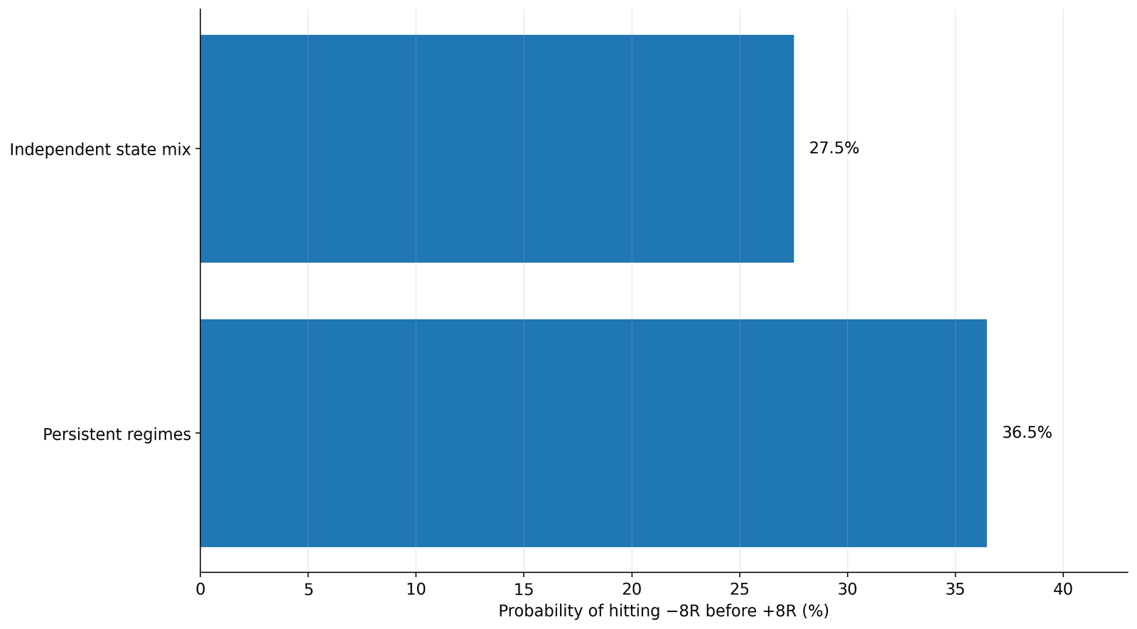
The illustration below holds the unconditional win probability at 53% with +1R/−1R outcomes. The independent version randomly redraws the favourable or adverse environment before every trade; the persistent version clusters those environments through a two-state Markov process. Across 50,000 simulated attempts with +8R and −8R barriers, persistent regimes produced a higher breach probability. This is an illustrative model, not an empirical estimate for any strategy.
4. Treat the nominal account size carefully
The headline account size is not the same as risk capital. A regime-sizing rule should be constrained by the distance to the binding loss floor, not simply multiplied by the nominal account value, which matters most for trailing structures.
A credible implementation workflow
- Define the decision. Decide whether the model controls total exposure, strategy activation, contract count, or only a warning dashboard.
- Choose the observation frequency. Daily data are more stable; intraday data create more observations but much more noise and microstructure dependence.
- Build causal features. Every feature must be available before the decision it influences.
- Separate training, validation and final testing. Hyperparameters must not be selected on the final period. Our note on reading research honestly and backtesting covers the guards.
- Generate online states. Use rolling or expanding estimation and preserve realistic delay.
- Compare against simple filters. Test realised-volatility thresholds, moving-average filters, drawdown throttles and fixed risk cuts.
- Integrate exact account mechanics. Daily resets, trailing floors, floating P&L, consistency rules and payouts must be modelled correctly.
- Stress the estimates. Vary the number of states, feature half-lives, transition persistence, costs, slippage and regime penalty.
- Monitor live drift. A regime model can fail because the state distributions themselves change.
Common backtesting errors
- Using smoothed historical states as though they were available live.
- Labelling regimes from the entire sample before splitting the data.
- Choosing the jump penalty from the final backtest.
- Ignoring the signal-to-trade delay.
- Assuming a good-looking regime chart proves economic value.
- Using the same data to invent features, choose the model and report performance.
- Fitting daily regimes and claiming they validate a five-minute strategy without a strategy-level test.
- Comparing only with buy and hold instead of simpler risk filters.
- Treating regime labels as objective truths rather than model-dependent estimates.
Practical conclusion
Hidden Markov models provide a formal way to infer persistent, unobserved market states from observable data. Their strongest trading application is adaptive risk: change exposure or strategy selection when the estimated distribution of returns and volatility has shifted. The 2024 Princeton study matters because it shows why persistence helps: a raw online HMM signal can switch too often to be practical, while the statistical jump model explicitly penalises transitions and, in three equity-index backtests, produced lower turnover, lower maximum drawdown and higher risk-adjusted performance than the HMM benchmark.
For prop-firm trading, the most promising use is not predicting tomorrow's direction. It is modelling when the trader's market or strategy enters an adverse state, reducing exposure before a loss cluster reaches a hard barrier, and building those persistent states into pass-rate and account-survival simulations.
A regime model does not need to predict the turning point to be useful. It needs to recognise that the distribution has changed before the new state stops persisting.
The final standard remains out-of-sample evidence. A regime model only adds value when it improves the real decision after costs, delay, estimation uncertainty and the exact prop-firm rules are included.
Model the risk, then test the odds
A regime filter is about surviving loss clusters, which is exactly what a prop challenge tests. Enter your win rate, reward-to-risk and risk per trade and estimate your odds of passing against a firm's real rules.
Open the pass rate simulator →New to prop firms? Start with the fundamentals.
Read the beginner's guide →Frequently asked questions
Can an HMM predict a crash?
Not reliably in the sense most traders mean. It can detect that recent observations increasingly resemble a high-volatility or adverse state. That detection normally follows the first part of the shift and may arrive late.
How many regimes should a trading model use?
Two states are interpretable and comparatively stable, but may combine very different conditions. Three states can represent calm, transition and crisis environments. The choice must be made through validation and stability analysis, not visual preference.
Should an HMM use market returns or strategy returns?
Use the data that correspond to the decision. A market-return HMM suits market exposure. A strategy-return model is more direct when the goal is to decide whether that strategy should stay active.
Is the jump model always better than an HMM?
No. The Princeton paper found better results for its selected features, markets and risk-overlay design. HMMs provide probabilistic outputs and a natural generative framework; jump models provide explicit persistence control. Both can fail through poor features, weak validation or changing market structure.
Can this be used on intraday futures?
Technically yes, but the paper's evidence is daily and long-only. Intraday testing must address session effects, overnight gaps, volatility around scheduled news, contract rolls, slippage and the much higher noise level.
References
Ang, A., & Timmermann, A. (2012). Regime changes and financial markets. Annual Review of Financial Economics, 4, 313–337.
Bemporad, A., Breschi, V., Piga, D., & Boyd, S. P. (2018). Fitting jump models. Automatica, 96, 11–21.
Bulla, J., Mergner, S., Bulla, I., Sesboué, A., & Chesneau, C. (2011). Markov-switching asset allocation: Do profitable strategies exist? Journal of Asset Management, 12, 310–321.
Hamilton, J. D. (1989). A new approach to the economic analysis of nonstationary time series and the business cycle. Econometrica, 57(2), 357–384.
Nystrup, P., Madsen, H., & Lindstrom, E. (2018). Dynamic portfolio optimization across hidden market regimes. Quantitative Finance, 18(1), 83–95.
Rabiner, L. R. (1989). A tutorial on hidden Markov models and selected applications in speech recognition. Proceedings of the IEEE, 77(2), 257–286.
Shu, Y., Yu, C., & Mulvey, J. M. (2024). Downside risk reduction using regime-switching signals: A statistical jump model approach. Journal of Asset Management, 25(5), 493–507.
FTMO. (n.d.). Trading objectives. Retrieved July 31, 2026, from ftmo.com/en/trading-objectives/
Topstep. (2026, June 24). Trading Combine parameters. help.topstep.com
Topstep. (2026, July 1). What is the Maximum Loss Limit? help.topstep.com