 DanFin
Drawdown in Trading: The Mathematics of Losing, Recovering, and Surviving Prop-Firm Limits
In short
- Drawdown is the drop from your equity's running peak, and it is path-dependent: the same trades in a different order can produce a very different worst drawdown.
- Recovery is asymmetric. A 10% drawdown needs an 11.1% gain and a 50% drawdown needs 100%, from the formula gain = drawdown / (1 − drawdown).
- Maximum drawdown is a single sample statistic, not a future ceiling. It grows with the observation window and with clustered, serially-correlated losses.
- A prop-firm loss limit turns drawdown into a barrier: the real question becomes whether you reach the profit target before the loss limit, which a positive-expectancy strategy can still fail.
- A firm's "maximum loss" rule is not the same as statistical maximum drawdown, and a static floor behaves differently from a trailing one.
Drawdown is not simply "being down". It is a path-dependent measure of how far an equity curve has fallen from a previous peak, how long capital stays underwater, and how hard the recovery problem becomes. In prop-firm evaluations it matters even more, because the path is constrained by explicit loss barriers.
The quick version: drawdown measures the decline from a previous equity peak, and maximum drawdown records the deepest such decline in a sample. But that single number does not tell the whole story: duration, recovery time, loss clustering, serial dependence, the length of the sample and the distribution of possible future drawdowns all matter. In a prop-firm evaluation a maximum-loss rule can act as an absorbing barrier: if equity touches the prohibited level before the profit target is reached, the attempt ends even if the strategy has positive long-run expectancy.
- What drawdown measures
- Depth, duration, time underwater
- Why recovery is asymmetric
- Why drawdown is path-dependent
- Drawdown vs volatility
- Why the horizon matters
- Serial correlation and clustering
- One max drawdown is not enough
- Conditional drawdown measures
- Drawdown, expectancy and survival
- Drawdown in prop-firm trading
- Monte Carlo and drawdown
- What the stats can and cannot tell you
- FAQ
Claim your spot on the waitlist
I am releasing one of my trading strategies shortly. Join the waitlist and receive a discount at launch.
Claim your spot →1. What drawdown actually measures
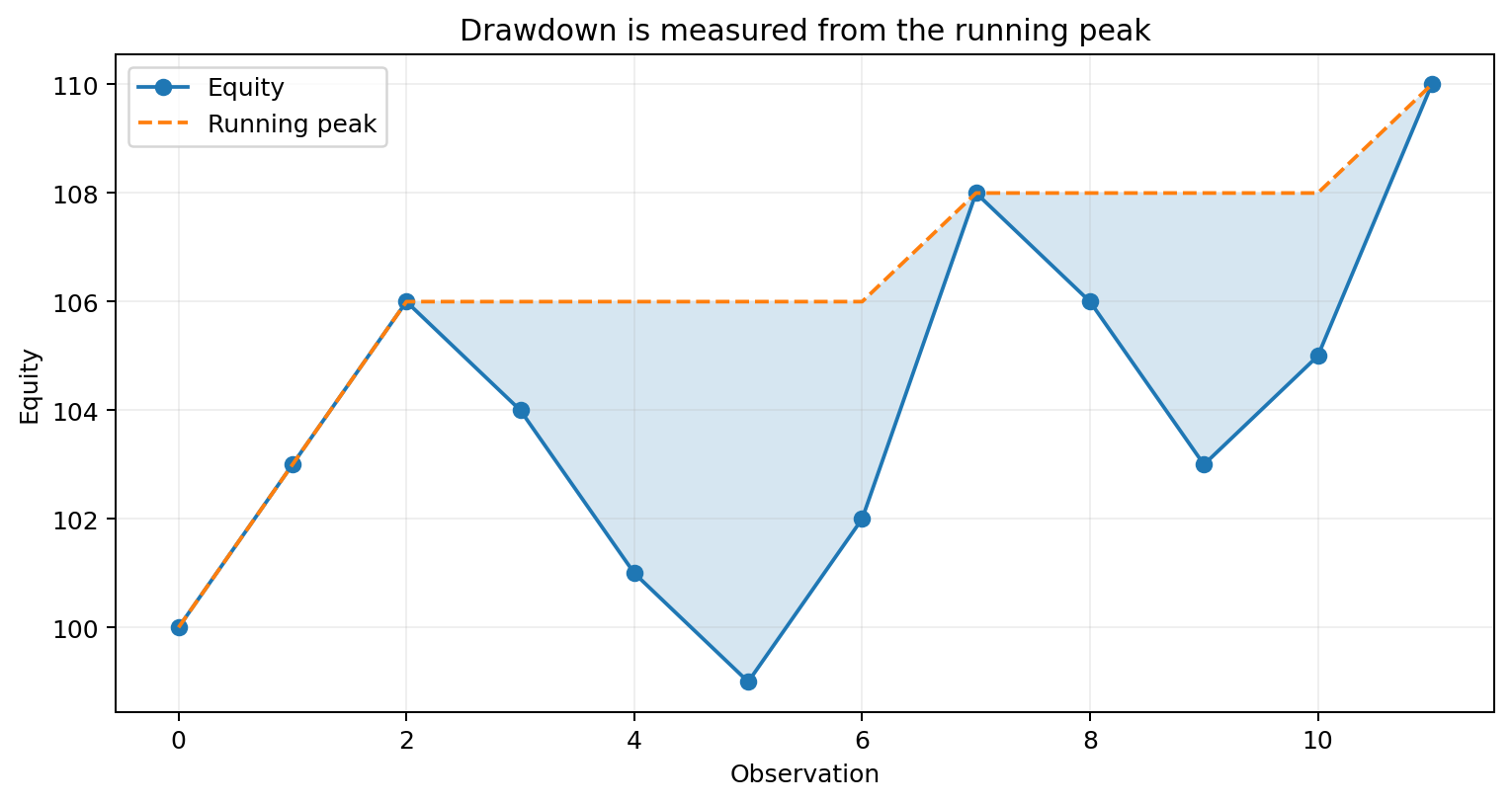
Suppose an equity curve is written Wₜ, the account value at time t. The running peak is the highest value achieved so far, and the percentage drawdown is how far you have fallen below it:
If an account reaches $100,000 and falls to $94,000 before making a new high, its drawdown is 6%. If it later reaches $105,000, the running peak resets, and a fall to $99,750 is a new 5% drawdown. Maximum drawdown (MDD) is the deepest peak-to-trough loss over the whole sample: MDD = max(Dₜ). This is why drawdown differs from a plain return. A return compares two points; drawdown continuously compares the current path with the best level previously achieved, so it carries information about the sequence of outcomes.
Magdon-Ismail, Atiya, Pratap and Abu-Mostafa (2004) formalised maximum drawdown for Brownian motion with drift and derived its distributional and asymptotic properties. Their work makes an important point clear: maximum drawdown is not a fixed attribute of a process, it is a random statistic generated by the path and the observation horizon.
2. Drawdown has more than one dimension
Traders often reduce drawdown to a single number, such as "a 7% maximum drawdown". That loses information. A drawdown episode has at least four dimensions:
| Dimension | Meaning | Why it matters |
|---|---|---|
| Depth | The peak-to-trough percentage decline | Measures the severity of the loss |
| Length | Time from peak to trough | Shows how quickly the loss accumulated |
| Recovery time | Time from trough back to the previous peak | Shows how long it took to repair the loss |
| Time underwater | Total time from the old peak until a new high | Combines decline and recovery into one meaningful duration |
Two strategies can both report a 10% maximum drawdown while imposing very different experiences: one falls 10% over three days and recovers in a week, the other declines gradually and stays below its old peak for a year. Maximum drawdown alone treats them as identical. This is why Bailey and Lopez de Prado (2015) studied both stop-out losses and time under water. Under their stylised assumptions the expected recovery period is about three times the period over which the loss accumulated, their "triple penance rule". It is a model-derived result, not a universal empirical law, but it highlights how recovery can take much longer than the decline that created it.
3. Why recovery is mathematically asymmetric
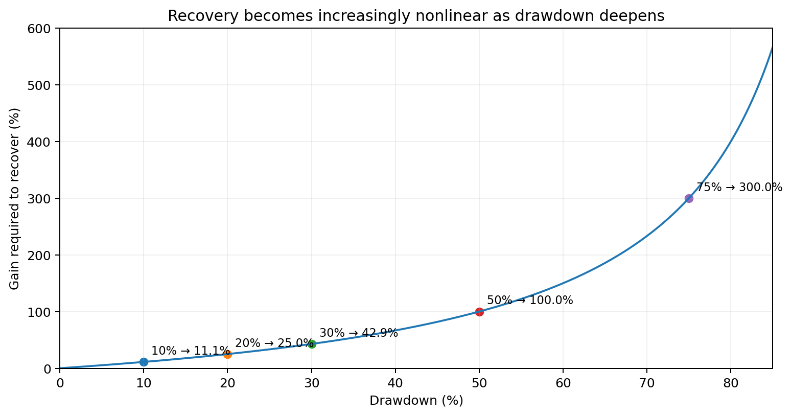
Percentage losses and gains are not symmetric, because a gain is applied to a smaller base after a loss. If a fraction d of capital is lost, the gain g needed to return to the peak satisfies (1 − d)(1 + g) = 1, which solves to:
| Drawdown | Gain required to recover |
|---|---|
| 5% | 5.26% |
| 10% | 11.11% |
| 20% | 25.00% |
| 30% | 42.86% |
| 40% | 66.67% |
| 50% | 100.00% |
| 75% | 300.00% |
This is pure arithmetic, not a forecast, and it does not mean a strategy in drawdown is likely to generate the required recovery. It simply states the percentage increase needed for equity to revisit the prior peak. You can put any drawdown into the free drawdown recovery calculator to see the exact gain required, and your odds of getting there before a limit.
4. Why drawdown is path-dependent
One of the most important properties of drawdown is path dependence. Consider two sequences that both contain three +$2 and three −$2 outcomes, both starting and finishing at 100, with identical total P&L. Sequence A alternates (+2, −2, +2, −2, +2, −2); Sequence B clusters the losses after the high (+2, +2, +2, −2, −2, −2). Sequence B creates a much deeper peak-to-trough decline, even though the individual outcomes and final P&L are exactly the same.
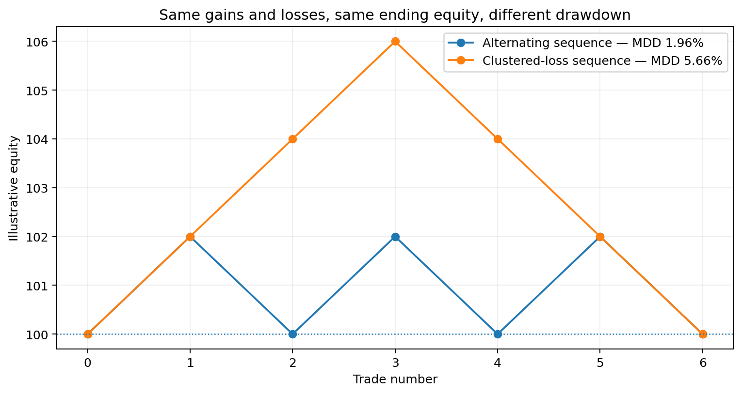
So drawdown cannot be reconstructed from the average return alone; it depends on when gains and losses occur relative to previous peaks. Goldberg and Mahmoud (2017) emphasise this and develop Conditional Expected Drawdown (CED), a risk measure based on the distribution of maximum drawdowns, showing that drawdown-based risk can react differently to serial correlation than volatility or Expected Shortfall.
5. Drawdown is not the same as volatility
Volatility measures the dispersion of returns around their mean; drawdown measures cumulative decline from a running high. A high-volatility process can move up and down around a rising trend without a long underwater period, while a low-volatility strategy can build a substantial drawdown from a run of small correlated losses.
| Risk statistic | Main object measured | Path-dependent? |
|---|---|---|
| Volatility | Dispersion of periodic returns | Usually no |
| Value at Risk (VaR) | A loss quantile for a set horizon | Usually no |
| Expected Shortfall (ES) | Average loss beyond a tail threshold | Usually no |
| Maximum drawdown | Largest peak-to-trough decline | Yes |
| Conditional drawdown measures | Tail or averaged properties of drawdown | Yes |
Goldberg and Mahmoud (2017) formalise CED as the tail mean of a maximum-drawdown distribution and show it is positively homogeneous and convex, useful properties for risk attribution. In their AR(1) exercises on US equity and bond data, CED is substantially more sensitive to the autoregressive parameter than volatility or Expected Shortfall, precisely because a path-based metric notices how returns cluster through time.
6. Maximum drawdown depends on the observation horizon
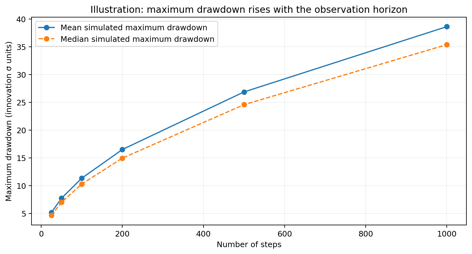
A historical maximum drawdown should never be read without asking: over what period? Extending a sample can never shrink its historical maximum drawdown, and stochastic theory predicts systematic horizon effects. For Brownian motion with drift, Magdon-Ismail et al. (2004) show the expected maximum drawdown grows logarithmically with time under positive drift, at a square-root rate under zero drift, and linearly under negative drift.
The exact Brownian model is an idealisation, but the lesson is robust: maximum drawdown is a sample statistic whose scale depends on how long the process is observed. Comparing a two-year backtest with a twenty-year backtest on maximum drawdown alone is not an apples-to-apples comparison.
7. Serial correlation and clustered losses
A basic Monte Carlo often assumes trades are independent and identically distributed. Real strategies may violate that through serial dependence, regime dependence, volatility clustering, overlapping positions or common factor exposure. Serial correlation matters for drawdown because losses that arrive close together accumulate before intervening gains repair the curve, deepening peak-to-trough losses without necessarily changing the average return.
Bailey and Lopez de Prado (2015) derive a stop-out framework under first-order serial correlation, and find that ignoring it can materially underestimate downside potential, by as much as 70% in their examples. That figure is specific to their model, but the conclusion generalises: IID assumptions are especially misleading when the quantity of interest is path-sensitive. The same theme appears in our pieces on volatility clustering and market regimes and loss clustering.
8. One historical maximum drawdown is not a forecast ceiling
Suppose a backtest reports an 8% maximum drawdown. It is tempting to say "the strategy's maximum drawdown is 8%". Statistically that is too strong: 8% is the maximum drawdown of one path over one finite period. A different ordering of trades, a different volatility regime, different correlations, a longer sample or different fills can produce another value. So maximum drawdown itself should be treated as a random variable, and a fuller analysis asks for a distribution: the median maximum drawdown across plausible paths, the shape of the upper tail, how often drawdown exceeds a threshold, how long severe drawdowns stay underwater, and how sensitive all of this is to dependence and regime assumptions. A single maximum drawdown is an observation; a drawdown distribution is a risk model. Our drawdown distribution guide shows what that looks like across many simulated attempts.
9. Beyond maximum drawdown: conditional drawdown measures
Maximum drawdown is intuitive but statistically severe: it focuses entirely on the single worst episode. Chekhlov, Uryasev and Zabarankin (2005) proposed a family of Conditional Drawdown measures that operate on the underwater curve, averaging the worst fraction of drawdowns rather than relying only on the single largest observation. The family links average drawdown (the typical underwater experience), conditional drawdown (a selected adverse tail) and maximum drawdown (the limiting worst case). This matters because two strategies can share the same maximum drawdown while behaving very differently beneath it: one isolated 10% event versus repeated 7 to 9% drawdowns. Goldberg and Mahmoud (2017) reach the problem from a related angle with Conditional Expected Drawdown, turning drawdown into a formal object for risk attribution and optimisation.
10. Drawdown, expected value and the survival problem
A positive expected return does not imply a smooth equity curve, nor does it guarantee that a finite path avoids a loss threshold. If a trade outcome X has positive expectation, E[X] > 0, that is an average over the assumed distribution; it does not specify the order in which outcomes arrive. A finite sequence can contain a long losing streak before the long-run average becomes visible. With unlimited capital the process may eventually recover; with a hard loss boundary, the sequence can end first. This is the bridge between expected value and survival: long-run profitability and short-run barrier survival are different statistical questions.
Busseti, Ryu and Boyd (2016) make this explicit in a Kelly framework. Classical Kelly maximises expected logarithmic growth; their risk-constrained version adds a bound on the probability of an undesirable drawdown, producing a formal trade-off between growth and drawdown risk (the same tension behind our Kelly calculator). Grossman and Zhou (1993) study portfolio choice under a drawdown constraint whose floor is a fraction of the maximum wealth so far, making the floor itself path-dependent, conceptually similar to trailing loss rules.
11. Why drawdown is structurally different in prop-firm trading
"Prop firm" is used broadly, rules vary across firms, products and account types, and many modern evaluations use simulated accounts. The discussion below is about the mathematical structure of loss limits, not whether any firm or account suits any trader.
11.1 A loss limit turns drawdown into a boundary condition
In an unconstrained backtest a drawdown is observed and the path continues. In an evaluation with a hard maximum-loss rule, reaching the prohibited level can terminate the attempt, which resembles a first-passage or barrier-hitting problem. With a profit target above the start and a loss boundary below it, the question is no longer just "is expected return positive?" but closer to "P(reach the profit barrier before the loss barrier)".
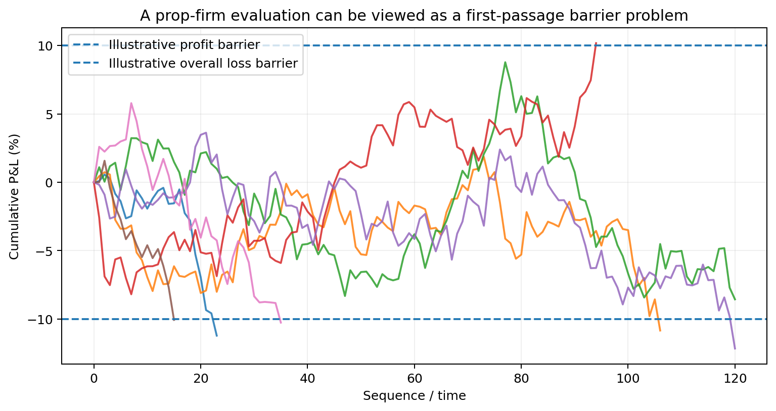
For a highly simplified arithmetic Brownian motion Xₜ = μt + σWₜ, starting at zero with an upper boundary +a and lower boundary −b, the probability of hitting the upper boundary first is:
This is an educational model, not a formula for a real challenge: real strategies have discrete trades, non-Gaussian outcomes, dependence, costs, varying exposure, daily rules and sometimes trailing boundaries. Its value is conceptual: barrier geometry changes the question from terminal return to path survival.
11.2 The nominal account size is not the loss budget
Consider a $100,000 account with a static 10% maximum overall loss. The nominal balance is $100,000, but the distance from the start to the prohibited loss boundary is $10,000. A $1,000 loss is therefore both 1% of the nominal account and 10% of the distance to the loss boundary. This does not mean $10,000 is the trader's economic capital at risk (fees, payouts and structure are separate), but it shows how percentages stated against the nominal size can hide how much of the drawdown buffer a loss consumes.
11.3 Daily loss limits add another path dimension
A total-loss floor is only one barrier; many evaluations also impose daily equity limits, creating dependence on intraday sequencing and the reset convention. As of 2 August 2026, FTMO's official 2-Step rules state a 5% Maximum Daily Loss and a static 10% Maximum Loss; the daily calculation is equity-based (including open P&L, swaps and commissions) and recalculated at 00:00 CE(S)T. FTMO's 2-Step Phase 1 profit target is 10% and Verification 5%. The5ers' High Stakes page, also checked on 2 August 2026, lists a 5% maximum daily loss and 10% maximum loss with a 10% and then 5% target. These are cited as examples and can change.
11.4 Static and trailing drawdown are not equivalent
A static floor stays tied to a fixed reference; a trailing floor can rise as the account makes new highs. That changes the geometry: a static boundary stays put while the target sits above, whereas a trailing boundary moves up after profitable periods, shrinking the future distance to the floor. FTMO's current 1-Step structure is a useful example: its 10% Maximum Loss operates on an end-of-day trailing basis (recalculated from the highest qualifying end-of-day balance, moving up but not down) with a 3% daily loss, which is mathematically different from its 2-Step static rule.
11.5 Positive expectancy can coexist with a low pass probability
A strategy may have positive long-run expectancy yet a meaningful chance of hitting a loss barrier before a profit target. The probability depends on far more than the mean: the variance and tail shape of outcomes, serial dependence and loss clustering, position overlap and correlation, the geometry of the barriers, daily versus total limits, static versus trailing floors, costs, and how exposure changes after gains and losses. This is why an evaluation cannot be judged from win rate and reward-to-risk alone: those are inputs to a model, but the outcome is generated by the full path. The free pass rate simulator runs thousands of those paths against a firm's rules to estimate the odds.
12. Monte Carlo: modelling a distribution of possible drawdowns
Monte Carlo methods replace one observed ordering with many possible paths, but the result is only as good as how those paths are generated. Simple trade reshuffling randomly permutes historical returns, revealing sequencing risk, but treats observations as exchangeable, so it destroys serial correlation, volatility regimes and overlapping trades if they exist. Bootstrap and block methods resample with replacement, and block bootstraps retain some short-range dependence by resampling adjacent groups. Parametric and regime models simulate from an estimated stochastic process, which can preserve dependence but introduces model risk.
For a prop evaluation, a simulation should not merely compute terminal P&L; it must test the path against the rules at each step, whether the total-loss or daily-loss threshold has been breached, whether a trailing floor has moved, whether the profit target is reached, and whether timing or minimum-day rules are satisfied. The output is a first-passage distribution: pass, fail, unresolved, time to termination, and maximum drawdown before termination. Crucially, a Monte Carlo engine does not create information absent from its inputs: if the return-generating process is wrong, the estimated pass probability can be wrong too.
13. What drawdown statistics can and cannot tell you
They can tell you how severe historical peak-to-trough losses were, how long recovery episodes lasted, how often the strategy spent time below previous peaks, how drawdown behaves across resampled or modelled paths, how close a simulated path comes to explicit loss barriers, and how sensitive it appears to sequencing and dependence.
They cannot, by themselves, tell you that a future maximum drawdown will stay below the historical maximum, that a strategy is profitable merely because drawdown is low, that a positive-expectancy strategy will pass an evaluation, that an IID Monte Carlo is valid when the process is dependent, that two firms with the same headline "10% max loss" have equivalent rules, or that a recovery percentage implies any probability or time to recovery. The central message: drawdown is a property of the path, not just the destination.
A rigorous drawdown report separates description from model-based estimate:
| Layer | Examples | Status |
|---|---|---|
| Historical description | MDD, average drawdown, underwater duration, recovery time | Observed in the sample |
| Distributional resampling | Bootstrap MDD distribution, shuffled-sequence MDD | Conditional on resampling assumptions |
| Parametric modelling | Brownian, AR, regime, stochastic-volatility simulations | Conditional on model specification |
| Barrier analysis | Probability of target before loss limit | Conditional on return model and exact rules |
This prevents a common error: presenting a simulation result as if it were an empirical fact. A model can estimate probabilities under assumptions; it cannot guarantee future path behaviour.
Calculate your recovery requirement
If an account is already in drawdown, the exact gain needed to recover the previous peak follows from the drawdown percentage. Enter yours and see it, plus your estimated odds of recovering before a loss limit.
Open the drawdown recovery calculator →Estimate your odds of passing a challenge against a firm's real rules.
Open the pass rate simulator →Frequently asked questions
What is drawdown in trading?
Drawdown is the percentage or dollar decline in equity from a previous running peak. If equity peaks at $100,000 and falls to $92,000, the current drawdown is 8%.
What is maximum drawdown?
Maximum drawdown is the deepest peak-to-trough decline observed in a specified sample. It is path-dependent and depends on the sample horizon.
Why does a 10% drawdown require more than a 10% gain to recover?
After a 10% loss, only 90% of the original capital remains. Recovering from 90 to 100 requires 10/90 = 11.11%.
Is maximum drawdown the same as a prop firm's maximum-loss rule?
No. Statistical maximum drawdown is normally measured from the running equity peak. A prop firm may define its loss threshold relative to initial capital, midnight balance, end-of-day highs or another contractual reference.
Can a positive-expectancy strategy still fail a prop-firm evaluation?
Yes. Positive expectancy describes an average under a probability model. A finite path can hit a hard loss boundary before a profit target, especially when variance, tails or serial dependence create adverse sequences.
Does risking a fixed percentage eliminate drawdown risk?
No. Percentage-based sizing changes how exposure scales with equity, but it does not remove losing sequences, path dependence or hard barrier risk.
Why is historical maximum drawdown not a reliable future ceiling?
It comes from one realised path and one observation window. A different sequence, regime or longer horizon can generate a larger drawdown.
What is time underwater?
Time underwater is the period between a previous equity peak and the moment that peak is finally recovered. It includes both the decline and the subsequent recovery.
References
Bailey, D. H., & Lopez de Prado, M. (2015). Stop-outs under serial correlation and the triple penance rule. The Journal of Risk, 18(2), 61–93.
Busseti, E., Ryu, E. K., & Boyd, S. (2016). Risk-constrained Kelly gambling. The Journal of Investing, 25(3), 118–134.
Chekhlov, A., Uryasev, S., & Zabarankin, M. (2005). Drawdown measure in portfolio optimization. International Journal of Theoretical and Applied Finance, 8(1), 13–58.
Goldberg, L. R., & Mahmoud, O. (2017). Drawdown: From practice to theory and back again. Mathematics and Financial Economics, 11(3), 275–297.
Grossman, S. J., & Zhou, Z. (1993). Optimal investment strategies for controlling drawdowns. Mathematical Finance, 3(3), 241–276.
Magdon-Ismail, M., Atiya, A. F., Pratap, A., & Abu-Mostafa, Y. S. (2004). On the maximum drawdown of a Brownian motion. Journal of Applied Probability, 41(1), 147–161.
Prop-firm rule examples (FTMO 2-Step, Trading Objectives and Maximum Daily Loss; The5ers High Stakes) were checked against official pages on 2 August 2026 and can change; verify current terms with the provider.